Fruit of Preterition

Contents

• I.a. Early/Late Training
• I.b. Universality and Robustness
• I.c. Pathology

Okay, so this is a list of surprising facts about how deep learning appears to work - the catalogue of mysteries. These observations are the walls against which I’ll be smashing mental models in a companion post. It also will hopefully serve double duty as a reference. There is every probability that some of these phenomena don’t generalize, are misinterpreted, don’t apply to LLMs etc. - I want to use them as a collection of weak evidences for a qualitative claim.

This is a lot of data so here’s a summary:

• There’s probably a qualitative difference between “early” and “late” training, with early training being more ‘formative’ than late training. Tentatively, early training sees ‘representation formation’, while late training ‘sharpens’ these representations. (§I.a)
• Lots of things appear to be architecture independent in a meaningful way, from example-difficulty or learning order, perhaps including even the overall structure of the learned representation. I forget who said this, but I’ve heard it said that “talking to Claude is talking to its training data”. (§I.b)
• Models are robust to really strange kinds of ablations, and this makes it hard to imagine a layer as secretly implementing one step of a boolean circuit. There’s probably an implicit tradeoff between ‘learning new computations’ and ‘denoising or becoming more confident in old ones’. (§I.b)
• Gradient flow (with no noise etc.) at least kinda works, so whatever our explanation is, it should at least kinda work if we assume that training can never cross a loss barrier. (§I.c)

I.a. Early/Late Training

First, there is a family of effects that suggest a difference between the ‘early’ and ‘later’ phases of training, with meaningfully different processes happening in either case. These are all things which point in this direction - to be clear, I do not contend they are the same thing, and some don’t clearly apply to LLMs. I merely wish to gesture at a pile of weak-moderate evidence that training is not ‘homogeneous’ - that it behaves differently at different times. Thus a mental model which cannot accommodate this cannot be correct.

Loosely, I think of the early phase as being like ‘learning representations’ and the latter phase as ‘sharpening’ them. A related idea I like is that of drift-diffusion transition from Tishby’s ‘Information Bottleneck’ (Stanford seminar on YouTube)¹, which imagines the forward and backward passes as sending a signal subject to some noise, with the transition occurring when the signal-to-noise ratio crosses one. In the early phase, gradient signal is high and optimization occurs normally. The latter phase begins when the gradient signal reaches the noise floor - then the network moves stochastically, occasionally lowering the noise floor by chance, and then optimizing until the newly resolvable signal is eaten.

Basin Commitment: The point in training at which SGD noise ceases to matter to the solution - in particular, the time \(t_{commit}\) such that networks cloned at time \(t' > t_{commit}\) with different batch noise will result in trained networks joined by a simple low-loss path. The region of parameter space occupied by these solutions is the final ‘basin’ of the model.²

Frankle et al. 2020, Fig. 3: instability (linear-interpolation error barrier) vs rewind step k, five networks.

(Linear, Layerwise) Mode Connectivity: Often, one can linearly interpolate (perhaps on a per-layer basis) between models cloned after \(t_{commit}\) without crossing a significant loss barrier. Kuditipudi, …, Arora, Ge shows this is a direct consequence of learned noise robustness. (I forget if they are equivalent or if the implication is unidirectional).

NTK Fit vs. Rotation: find this and write it. I forget the evidence for this.

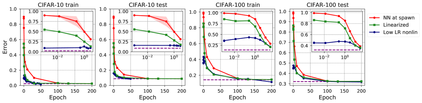Fort et al. 2020, Fig. 8: linearized training started at epoch t̃ (green) vs full nonlinear training (red); the gap closes after the first few epochs.

Breakeven Point: There is a single point in training at which models trained at different learning rates (LRs) qualitatively diverge - larger LR models end up with lower spectral norm and better generalization etc. If I understand correctly this is synonymous with the activation of the edge of stability phenomenon (when the largest Hessian eigenvalue becomes greater than 2/LR, the stability threshold for discretized gradient descent); Central flows uses secular perturbation theory to show how this qualitatively changes the trajectory and results in flatter solutions.³

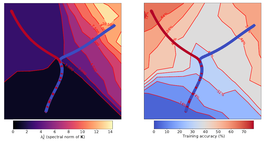Jastrzębski et al. 2020, Fig. 1: UMAP of early trajectories for two LRs, coloured by gradient-covariance spectral norm and train accuracy.

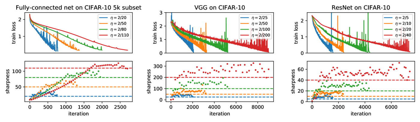Cohen et al. 2021, Fig. 1: train loss and sharpness; sharpness rises to 2/η and hovers there.

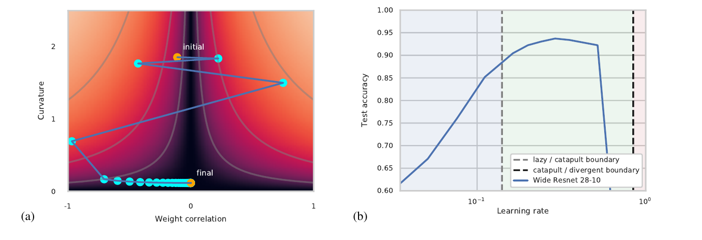Lewkowycz et al. 2020, Fig. 1: the catapult trajectory and test accuracy vs learning rate.

Model Averaging: for a training trajectory \(\theta(t)\), there exists a time \(t_{av}\) such that averaging together checkpoints taken after \(t_{av}\) produces a functional model (occasionally with better loss - this is related to the more classical Polyak averaging, see Goodfellow, Bengio & Courville §8.7.3). I believe at least some production LLMs have done this or a complicated version of it. The intuition is that if there’s a sharp pit in the loss-landscape, the trajectory probably bounces around this rather than going ‘in’, so the average should be closer. In our language, the ‘late’ loss-landscape is flat and so steps are noisier - note this isn’t batch noise so much as the landscape just being low-frequency, low-amplitude; we imagine that averaging the checkpoints helps (retroactively) ‘triangulate’ the direction the model should have moved. There’s a cute interpretation: for \(\bar \theta := \frac{1}{M}\sum_{n=1}^{M} \theta_{t_0 + n \Delta t}\), you imagine each step to have a slowly changing drift component, and a stochastic diffusion component, and you want to choose \(t_{\text{diffusion}} \lesssim \Delta t \lesssim t_{\text{drift}}\).

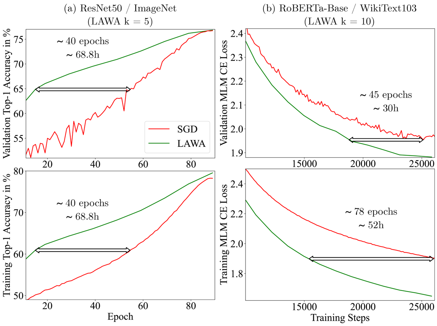Kaddour 2022 (LAWA), Fig. 1: latest-weight-averaging vs SGD on ResNet50/ImageNet and RoBERTa/WikiText103.

Emergence of Activation Plateaus and Cell Structure⁴. This is something I and a collaborator have been thinking about a lot, and I hope to have a post on soon. Tl;dr, if you take three activation vectors and draw the plane that passes through them, then look at the image of that plane, you tend to see the outputs change only across a thin boundary, rather than interpolate smoothly - the activations seem to be arranged in Voronoi-like cells - an emergent digital code. Tentatively, with details forthcoming, these cells seem to form quite early in training and sharpen over time - some significant portion of training is spent on this sharpening, corresponding to more confident predictions (implicit bias of GD). They seem to be more prominent in larger models.

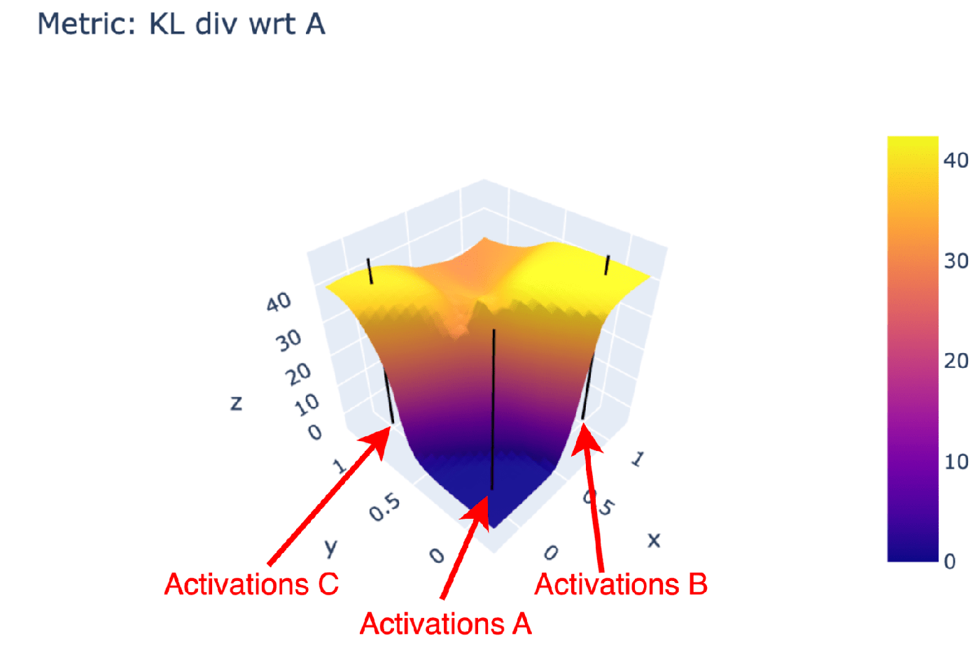Heimersheim & Mendel 2024: KL divergence of the output over the plane through three activations; flat plateaus with sharp walls.

Hessian Spectra: At initialization, the Hessian eigenvalues are random, but they very rapidly change to have a characteristic structure: a few large-positive-curvature directions, many near-neutral directions, and a few lightly negative-curvature directions. I’ve talked before (here) about the parallel to the fitness-effect-of-mutation distribution in biology. Part of this may be idiosyncratic to the classification objective, but the qualitative picture extends to LLMs⁵. I don’t know enough about this yet, but it also seems to be true that the Hessian is nearly block-diagonal per-layer⁶ - which implies that layers are nearly independent of one another. Probably this is only directionally true, but it seems noteworthy. See below on the ‘painters’ view as well.⁷

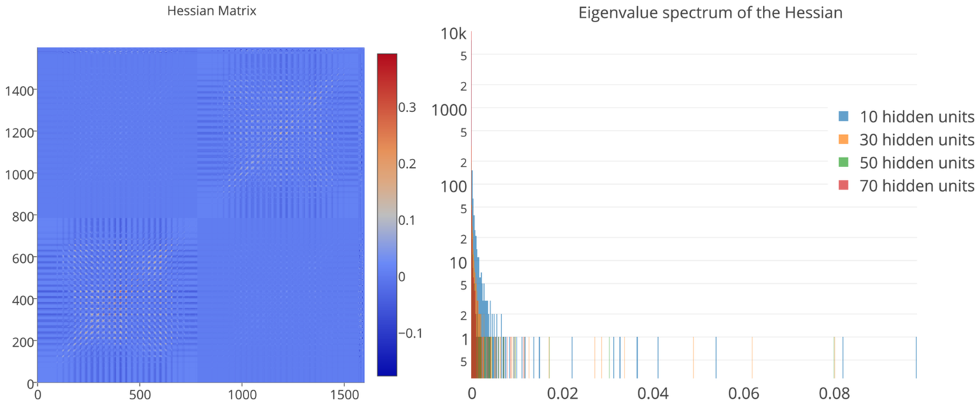Sagun et al. 2016, Fig. 1: Hessian and its eigenvalue histograms, a bulk at zero plus a few outliers (panels composited).

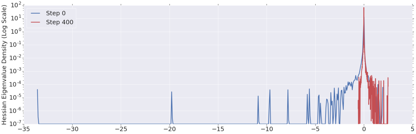Ghorbani et al. 2019, Fig. 2: Hessian spectral density at step 0 vs step 400; the negative eigenvalues vanish.

Critical Periods: Vision networks shown distorted training data for part of training recover much better if the distortion is later rather than earlier; the deficit is worse as the distortion is maintained for longer. There’s a qualitative similarity to critical periods in optic development and amblyopia in animals. Iirc this can be a bit finicky depending on LR and optimizer, so it’s maybe not that universal. The metric they measure, the Fisher trace, is closely related to the Hessian, and so this can be predicted from that. Qualitatively (with \(f\) the network outputs, \(J = \partial f / \partial \theta\), and \(\ell\) the per-example loss),

\[H \;=\; \underbrace{\mathbb{E}\!\left[J^\top \big(\nabla_f^2 \ell\big) J\right]}_{\text{Gauss-Newton}\;\approx\;\text{Fisher}} \;+\; \underbrace{\mathbb{E}\!\left[\sum_k \frac{\partial \ell}{\partial f_k}\, \nabla_\theta^2 f_k\right]}_{\text{residual}\,\times\,\text{curvature of } f}\]

later in training, the residuals \(\partial \ell / \partial f_k\) are small, so the Hessian is roughly the Fisher.

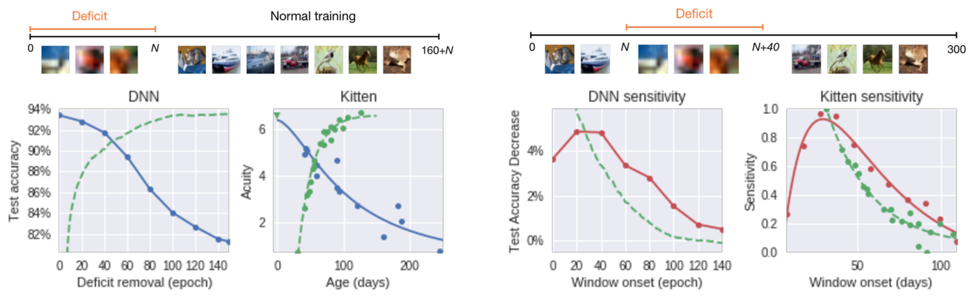Achille, Rovere & Soatto 2019, Fig. 1: final accuracy vs the epoch at which the blur deficit is removed, beside the kitten data.

I.b. Universality and Robustness

In this section, I’ll point to a few phenomena that suggest there is a meaningful universality to what models learn, often independent of training objective, architecture, etc. I’ll add a few miscellaneous puzzling comments about the layerwise structure of learning in transformers. These should all be taken with quite the grain of salt (most of them are controversial, but I think they’re pointing at something real, even if their particular claims are refuted), but the fact that human brains reliably implement the same functionality should set our priors to thinking this is at least limitedly true.

Platonic Representation Hypothesis: by far the most enticing and controversial claim on this list is the idea that models, even across modalities, learn the same structures and organize them similarly. The evidence for this is something of the form ‘the k-nearest-neighbors of this point in modality A are the same as the k-nearest neighbors of the corresponding point in modality B’, plus some other stuff about downstream finetuning. Margot’s ‘An Ontology of Representations: Limits of Universality’ is a good discussion on how seriously to take this claim’s implications, supposing it is strongly-true. This is methodologically related to CKA and (SV)CCA analyses, which analyze how these representations change between layers.

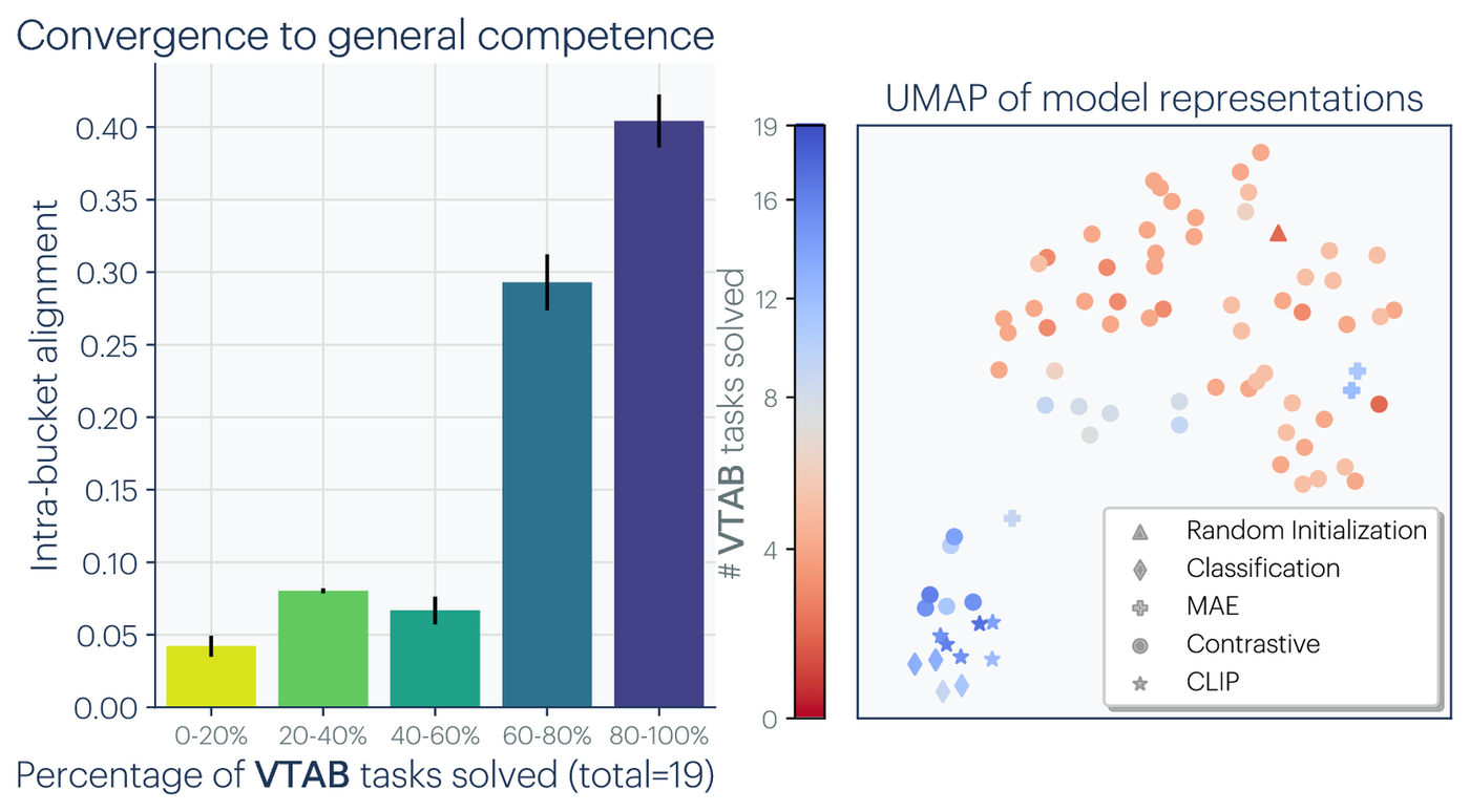Huh et al. 2024, Fig. 2: representational alignment rises with competence (VTAB tasks solved); panels composited.

Model Stitching: If you cut two models in half and form a chimera (fitting a linear adapter from one residual stream to another), the result seems to work reasonably well. This applies mainly for the middle layers of transformers, and doesn’t seem to work for the later or earlier layers. This suggests that the partially-completed computations are interchangeable between models. Think how strange this would be for circuit-boards or python programs!

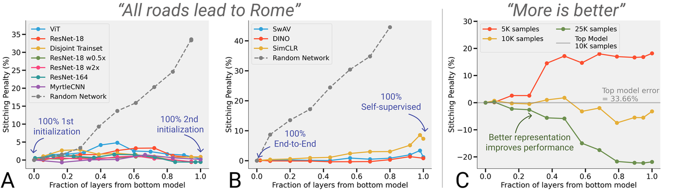Bansal, Nakkiran & Barak 2021, Fig. 2: stitching penalty vs fraction of layers.

Critical Layers: We observe that if we reset a given layer to its value at initialization (or just early in training), some layers disproportionately affect the loss while others seem not to matter. Looking at the numbers, it’s possible this is just normalization layers or something architectural rather than a true phenomenon - it survives in my mind in light of the latter.

Zhang, Bengio & Singer 2019, Fig. 1: per-layer re-randomization / re-initialization robustness, MNIST FCN (panels composited).

Painters: They claim that if you take a transformer’s middle layers one can generally repeat a layer, reverse them etc. with minimal reduction in loss, sometimes with some gain. The “painters” idea is that ‘each layer is a painter which adds its own brushstroke to the canvas’ lol. I expect this to be related to how looping transformers⁸ work, as well as to the earlier-discussed cell structure. My best understanding of this is that these layers are at least sorta doing ‘error correction’, or some sort of cleanup. Iirc there’s a claim that this sort of fuckiness differentially harms hard math/coding benchmarks - if so it’d suggest that reasoning ability may be bottlenecked by this sort of error-correction. Intriguing but I’m a bit dubious that there’s a straightforward relationship.

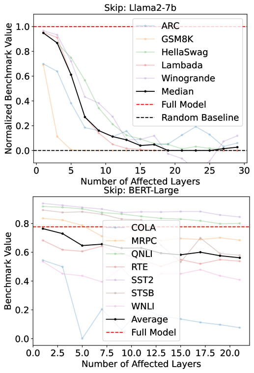Sun et al. 2024, Fig. 4: accuracy when a single middle layer is skipped, Llama2-7B (top) and BERT-Large (bottom).

Two things that didn’t make it in because I haven’t formed a coherent picture of what’s important yet: 1. learning order of different samples, with possible patterns in ‘universally’ hard samples, and 2. distillation, its scaling laws, and behavioural pathologies.

I.c. Pathology

REWORD THIS and REFORMAT WITH BOLDING ETC.

We know that evolution and gradient descent obey a principle of intermediate use - complex assemblies must be made of components which are themselves sufficiently useful to not be selected away. I previously spent a lot of time doing mental gymnastics to figure out how evolution could be effectively non-myopic due to noise effects, because I figured there was no hope of recovering complex sequential algorithms if we so constrained intermediate steps. While this non-myopia certainly happens occasionally in evolution, this doesn’t seem plausible to me as a ‘sine qua non’ for what is happening when we do SGD.

Importantly, we observe that ideal gradient flow (full-batch, low-LR, no-EoS) training at least kinda works⁹, and full-batch on GPT2 (Shawn Hu) also still kinda-works - whatever is happening, it seems likely that true noiseless gradient-flow (i.e., with no ‘selective slack’) is doing qualitatively the same thing, just awfully. This means that a belief in “circuits” would require us to believe that we can have the network do this stagewise learning without ever hitting a meaningful barrier in the loss landscape. This is hard for me to imagine for even the rudimentary “change wire A→B to be A→C” operation.

Another thing that seems to make the above more confusing is the apparent importance of plasticity - models seem to degrade in ‘plasticity’ as you train longer, which feels contradictory to the idea that they should be growing more circuits which generalize better. If one thinks of training as the elution of these circuit assemblies, we would of course predict that models with ‘more and deeper’ circuit assemblies should be easier to finetune. It also seems relevant to how LoRA adapters learn and forget.

TODO WRITE SECTION: LoRA vs Full Fine-tuning: An Illusion of Equivalence

---