[AI-Written] Information in Continua I: Functions as Signals

Author’s note. This three-part series is a writeup of a kernel-based analogue of information theory I have been developing over the course of my research at MATS and the Iliad Fellowship. It has taken on enough substantive form that I’m pleased to share it. The motivation is to develop an analogue of information theory which is better suited to the description of continuous spaces and computations thereon. This permits a native notion of ‘resolution’ and ‘imprecision’. The particular problem I wanted to resolve is that, for a function (f(x)), we can only measure it at finite resolution, so fluctuations on unresolved scales could in principle carry large amounts of information, and to do this in a way that permits treating these fluctuations and noise on a distinct footing. Because of this resolution-centered perspective, I expect the theory to be useful for probing information in functions, as the objects are well-suited for spectral approximation.

The theory starts by developing a function-space analogue of channel-capacity in part I, extends this to a notion of resolution-bounded probability in part II, and in part III develops an application to continuous-space computations.

I decided to have GPT5.5-Pro write these up, judging that it was less likely to make mistakes than me. I apologize in advance for any cringe.

Research context. This work was developed during MATS 9.1 under Richard Ngo and during the Iliad Fellowship under Dmitry Vaintrob.

1. The Object

Classical information theory begins with messages and a noisy channel. The standard discrete entropy of a random variable asks how many bits are needed to identify which symbol occurred. For continuous variables, the corresponding objects are more delicate: differential entropy is coordinate-dependent, binning introduces an arbitrary resolution, and arbitrarily fine fluctuations can dominate the count.

The object I want here is different. Suppose we have a space of states (X), and suppose we can ask real-valued questions about those states. A question is a function

\[f:X\to \mathbb R.\]

The function (f) is the signal. A measurement process does not see all possible functions equally well. Some functions are smooth and cheap. Some are rough and expensive. Some are hidden below the noise floor. The proposed information measure is therefore not:

\[\text{how many states are there?}\]

but:

\[\text{how many affordable functions are distinguishable at the available resolution?}\]

This post develops the corresponding channel-capacity object. Part II uses the same geometry to define precision-bounded beliefs. Part III uses it to decompose continuous-space computations.

2. Observable Spaces

Let (k) be a positive definite kernel on (X). By the Moore-Aronszajn theorem, (k) determines a unique reproducing kernel Hilbert space (\mathcal H_k) of functions on (X). The reproducing property is

\[f(x)=\langle f,k(x,\cdot)\rangle_{\mathcal H_k}.\]

The RKHS norm is a complexity geometry on questions. For example, an RBF kernel makes smooth functions cheap relative to spiky functions, while a Matérn kernel changes the roughness scale being penalized. More generally, take a positive self-adjoint operator

\[L:\mathcal H_k\to\mathcal H_k\]

and define functional energy by

\[E(f)=\langle f,Lf\rangle_{\mathcal H_k}.\]

The energy ball is

\[B_E(P)=\{f\in\mathcal H_k:E(f)\le P\}.\]

This is the analogue of a power constraint. We are not allowing every measurable question. We are allowing questions that fit inside a specified functional budget.

3. Observation and Resolution

A function is not automatically observed. We need an observation operator

\[A:\mathcal H_k\to\mathcal Y,\]

where (\mathcal Y) is a Hilbert space of observable outputs. Two examples are enough to anchor the construction.

For finite samples (x_1,\ldots,x_n),

\[Af=(f(x_1),\ldots,f(x_n))\in \mathbb R^n.\]

For a population measure (\mu),

\[A=J_\mu:\mathcal H_k\to L^2(\mu),\qquad J_\mu f=f.\]

Noise or resolution also lives in the output space. Let

\[N:\mathcal Y\to\mathcal Y\]

be a positive covariance operator. The noisy observation is

\[Y=Af+\eta,\qquad \eta\sim (0,N).\]

Whitening output differences by (N^{-1/2}) measures them in noise units. Energy-normalizing functions by (L^{-1/2}) measures input directions in power units. The normalized channel is

\[S=N^{-1/2}AL^{-1/2}.\]

Its type signature is

\[S:\mathcal H_k\to\mathcal Y.\]

Interpretation:

\[S=\text{observable output in noise units per unit functional energy.}\]

Standing analytic assumptions. The formulas below are literal in finite dimension. In infinite dimension, read them under the standard compact-operator assumptions: (L) and (N) are strictly positive on the relevant subspaces, (L^{-1/2}) and (N^{-1/2}) are interpreted on their domains or as pseudoinverses on quotient spaces, (S=N^{-1/2}AL^{-1/2}) is compact, and (SQS^\ast) is trace class for the admissible input covariances (Q). The empirical kernel-matrix case satisfies the finite-dimensional version after regularization.

4. Signal-to-Noise Modes

The singular values of (S) are the basic spectral data. Write

\[S^\ast S u_i=\rho_i u_i,\]

with (\rho_i\ge 0). The (\rho_i) are squared signal-to-noise gains.

In original function coordinates (v_i=L^{-1/2}u_i), this becomes the generalized eigenproblem

\[A^\ast N^{-1}A v_i=\rho_i L v_i.\]

Proposition 1. The modes (v_i) are the functions that maximize observed signal-to-noise per unit energy, subject to orthogonality to earlier modes.

Proof. For (f=L^{-1/2}u),

\[\frac{\|Af\|_{N^{-1}}^2}{E(f)} = \frac{\|N^{-1/2}AL^{-1/2}u\|^2}{\|u\|^2} = \frac{\langle u,S^\ast S u\rangle}{\langle u,u\rangle}.\]

The Rayleigh-Ritz variational theorem says this quotient is maximized by the top eigenvector of (S^\ast S), and subsequent constrained maxima are the later eigenvectors. Rewriting (u=L^{1/2}v) gives the generalized eigenproblem. (\square)

For finite data with (Af=(f(x_1),\ldots,f(x_n))), (L=I), and (N=\sigma^2 I), the nonzero (\rho_i) are proportional to the eigenvalues of the kernel Gram matrix:

\[\rho_i=\frac{\lambda_i(K)}{\sigma^2}, \qquad K_{ab}=k(x_a,x_b),\]

up to the convention-dependent normalization of (K). The empirical question is therefore spectral: how many kernel modes of the dataset remain visible above the noise floor?

5. Capacity Entropy

There are two closely related capacity objects.

The hard object is a covering entropy. In finite dimension, consider the observed image of the energy ball:

\[N^{-1/2}AB_E(P).\]

This is an ellipsoid in whitened observation space. If (S) has squared singular values (\rho_i), then the axes of this ellipsoid have lengths (\sqrt{P\rho_i}). At resolution (\varepsilon), the logarithm of the covering number is approximately

\[H^{\mathrm{hard}}_\varepsilon(P) \approx \sum_i \log_+\left(\frac{\sqrt{P\rho_i}}{\varepsilon}\right).\]

This is the usual ellipsoid-covering estimate, ignoring boundary constants. In infinite dimension it requires compactness and tail control. The qualitative content is that only modes whose observable amplitude exceeds the resolution contribute.

The soft object is the Gaussian channel-capacity analogue. Let (Q\succeq 0) be an input covariance in energy-normalized coordinates, with

\[\operatorname{tr}(Q)\le P.\]

Define

\[C_{\mathrm{RKHS}}(P;A,N,L) = \sup_{Q\succeq 0,\operatorname{tr}(Q)\le P} \frac12\log\det(I+SQS^\ast).\]

Spectrally,

\[C_{\mathrm{RKHS}}(P) = \frac12 \sup_{p_i\ge 0,\sum_i p_i\le P} \sum_i\log(1+p_i\rho_i).\]

The optimum is water filling:

\[p_i^\ast=\left(\tau-\frac1{\rho_i}\right)_+,\]

where (\tau) is chosen so that (\sum_i p_i^\ast=P).

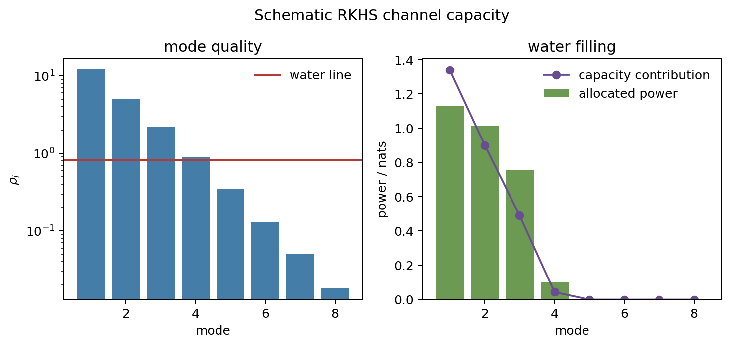
Figure 1. A schematic finite-dimensional capacity calculation. The (\rho_i) are mode qualities of the normalized channel (S=N^{-1/2}AL^{-1/2}). Water filling allocates power only to modes whose signal-to-noise gain is high enough.

Proposition 2. For fixed singular values (\rho_i), the optimizing covariance (Q) is diagonal in the right singular basis of (S), and its diagonal entries obey the water-filling rule above.

Proof. Take an SVD (S=U\Sigma V^\ast). By unitary invariance of trace and determinant, write (\widetilde Q=V^\ast QV). Then

\[\log\det(I+SQS^\ast) = \log\det(I+\Sigma \widetilde Q\Sigma^\ast).\]

For fixed diagonal entries of (\widetilde Q), Hadamard’s determinant inequality is maximized by a diagonal positive semidefinite matrix. Thus the problem reduces to

\[\max_{p_i\ge 0,\sum p_i\le P}\sum_i \frac12\log(1+p_i\rho_i).\]

The KKT conditions give

\[\frac{\rho_i}{1+p_i\rho_i}=2\lambda\]

on active modes, hence (p_i=\tau-1/\rho_i) for (\tau=1/(2\lambda)), and (p_i=0) when this expression is negative. (\square)

This is the function-space analogue of Gaussian channel capacity. A bounded system spends energy only on modes that buy distinguishability.

6. Data Processing Requires the Right Noise Geometry

The natural data-processing statement is:

\[\text{post-processing cannot create new distinguishable low-energy functions.}\]

This is true only when the downstream noise geometry is inherited from the upstream experiment. If we take an output (Y), apply a deterministic map (R), and then declare a tiny new noise covariance on (RY), we have changed the measurement problem.

In the linear case, suppose

\[Y=Af+\eta,\qquad \eta\sim(0,N_Y),\]

and

\[Z=RY.\]

Then

\[Z=RAf+R\eta,\]

so the induced downstream noise covariance is

\[N_Z^{\mathrm{ind}}=RN_YR^\ast.\]

If (R) is non-invertible, this is a quotient geometry on the retained directions, with inverse covariance understood as a pseudoinverse on (\operatorname{im} R). Directions discarded by (R) cannot be recovered. Directions retained by (R) inherit their uncertainty from upstream.

Proposition 3. If

\[R^\ast N_Z^{-1}R\preceq N_Y^{-1},\]

then

\[C(P;RA,N_Z,L)\le C(P;A,N_Y,L).\]

Proof. The inequality says that every downstream output difference, pulled back to the upstream space, is no more distinguishable than it was upstream:

\[\|Ry\|_{N_Z^{-1}}^2 = \langle y,R^\ast N_Z^{-1}Ry\rangle \le \langle y,N_Y^{-1}y\rangle = \|y\|_{N_Y^{-1}}^2.\]

Therefore

\[(N_Z^{-1/2}RA)^\ast(N_Z^{-1/2}RA) \preceq (N_Y^{-1/2}A)^\ast(N_Y^{-1/2}A).\]

After energy normalization,

\[L^{-1/2}A^\ast R^\ast N_Z^{-1}RA L^{-1/2} \preceq L^{-1/2}A^\ast N_Y^{-1}A L^{-1/2}.\]

For any admissible input covariance (Q\succeq 0), Loewner monotonicity of (\log\det(I+\cdot)) on positive trace-class operators gives

\[\log\det(I+N_Z^{-1/2}RAQ A^\ast R^\ast N_Z^{-1/2}) \le \log\det(I+N_Y^{-1/2}AQ A^\ast N_Y^{-1/2}).\]

Taking the supremum over the same feasible set of (Q)’s gives the capacity inequality. (\square)

This is the clean data-processing principle: post-processing cannot increase capacity when downstream distinguishability is measured using the noise geometry induced by the original experiment.

7. What This Is Not

This object is not the Shannon entropy of a binned continuous variable. It does not count occupied bins. It counts distinguishable low-energy functions.

It is also not MMD. The maximum mean discrepancy compares two distributions by

\[\operatorname{MMD}(P,Q) = \sup_{\|f\|_{\mathcal H}\le 1} \left(\mathbb E_P f-\mathbb E_Q f\right).\]

That is a distance between distributions. RKHS capacity instead fixes an observation process and asks for the dimension and strength of the function modes it can distinguish. In the population case (A=J_\mu), it depends on the spectrum of the kernel integral operator under (\mu), not merely on the mean embedding of (\mu).

Nor is it a semantic theory by itself. A kernel, energy, observation operator, and noise geometry define a measurement problem. If those choices correspond to questions we care about, the resulting capacity says something about those questions. The formalism does not attach meaning to modes without that prior specification.

8. Summary

The construction has four ingredients:

1. a space of observables (\mathcal H_k);
2. an energy geometry (L);
3. an observation channel (A);
4. a noise or resolution geometry (N).

Together they define the normalized channel

\[S=N^{-1/2}AL^{-1/2}.\]

The singular values of (S) are the observable signal-to-noise modes. Covering entropy counts how many modes exceed a resolution threshold. Gaussian capacity allocates finite power across those modes by water filling.

Part II uses this same object to define a bounded form of belief. Instead of assigning probabilities to all measurable events, a bounded agent assigns expectations to affordable questions.

References

• Shannon, C. E. “A Mathematical Theory of Communication.” Bell System Technical Journal, 1948. Reprint hosted by Harvard: https://people.math.harvard.edu/~ctm/home/text/others/shannon/entropy/entropy.pdf.
• Cover, T. M. and Thomas, J. A. Elements of Information Theory. Wiley, 2006.
• Aronszajn, N. “Theory of Reproducing Kernels.” Transactions of the American Mathematical Society, 1950.
• Berlinet, A. and Thomas-Agnan, C. Reproducing Kernel Hilbert Spaces in Probability and Statistics. Kluwer, 2004.
• Schölkopf, B. and Smola, A. J. Learning with Kernels. MIT Press, 2002.
• Gretton, A., Borgwardt, K., Rasch, M., Schölkopf, B., and Smola, A. “A Kernel Method for the Two-Sample Problem.” arXiv:0805.2368, https://arxiv.org/abs/0805.2368.
• Muandet, K., Fukumizu, K., Sriperumbudur, B., and Schölkopf, B. “Kernel Mean Embedding of Distributions: A Review and Beyond.” arXiv:1605.09522, https://arxiv.org/abs/1605.09522.

LLM Usage

The source conversation for Parts I and II was https://chatgpt.com/share/6a4bdbee-c8d8-83eb-a58d-38b213087b2f. This post was written with assistance from GPT5.5-Pro and Codex. Any errors are my responsibility.