[AI-Written] Information in Continua II: Precision-Bounded Beliefs

Author’s note. This three-part series is a writeup of a kernel-based analogue of information theory I have been developing over the course of my research at MATS and the Iliad Fellowship. It has taken on enough substantive form that I’m pleased to share it. The motivation is to develop an analogue of information theory which is better suited to the description of continuous spaces and computations thereon. This permits a native notion of ‘resolution’ and ‘imprecision’. The particular problem I wanted to resolve is that, for a function (f(x)), we can only measure it at finite resolution, so fluctuations on unresolved scales could in principle carry large amounts of information, and to do this in a way that permits treating these fluctuations and noise on a distinct footing. Because of this resolution-centered perspective, I expect the theory to be useful for probing information in functions, as the objects are well-suited for spectral approximation.

The theory starts by developing a function-space analogue of channel-capacity in part I, extends this to a notion of resolution-bounded probability in part II, and in part III develops an application to continuous-space computations.

I decided to have GPT5.5-Pro write these up, judging that it was less likely to make mistakes than me. I apologize in advance for any cringe.

Research context. This work was developed during MATS 9.1 under Richard Ngo and during the Iliad Fellowship under Dmitry Vaintrob.

1. Belief as Ability to Answer Questions

Part I replaced information over bins with capacity over observable functions. The same move changes how probability should look for bounded systems.

Classical probability starts with a measure (\mu) on a state space (X). It then assigns expectations to bounded measurable functions:

\[b_\mu(q)=\mathbb E_\mu[q]=\int_X q(x)\,d\mu(x).\]

For a bounded agent, the expectation functional is often the operational object. The agent is not given arbitrary measurable events at infinite precision. It has a question space, a cost geometry, and a resolution limit.

So define a belief as a positive normalized linear functional

\[b:\mathcal Q\to\mathbb R,\]

where (\mathcal Q\subseteq \mathcal H_k) is a space of representable questions. Positivity and normalization mean

\[q\ge 0 \Rightarrow b(q)\ge 0,\qquad b(\mathbf 1)=1,\]

whenever the constant function (\mathbf 1) belongs to (\mathcal Q). If (b=b_\mu) for some measure (\mu), this recovers ordinary probability on the questions in (\mathcal Q). The difference is that (\mathcal Q) need not contain all measurable indicators.

The mental primer is simple: a bounded belief is not a hidden full posterior. It is a rule for answering the questions the system can afford to represent.

2. Precision Distance

Let the question space have an energy (E(q)). At budget (P), define the induced question distance

\[d_P(\mu,\nu) = \sup_{E(q)\le P} |\mathbb E_\mu q-\mathbb E_\nu q|.\]

At resolution (\epsilon), write

\[\mu\sim_{P,\epsilon}\nu \quad\Longleftrightarrow\quad d_P(\mu,\nu)\le \epsilon.\]

For (\epsilon>0), this is not generally transitive, so it is not an equivalence relation. It is a finite-resolution indistinguishability threshold. The true quotient appears at (\epsilon=0), where (d_P(\mu,\nu)=0). This distinction matters: finite precision gives overlapping balls, not a canonical partition.

The distance depends on the question geometry. If (\mathcal H_k) contains smooth functions and (E) penalizes roughness, then high-frequency differences between (\mu) and (\nu) are invisible at low budget. If (P\to\infty) and (\epsilon\to 0), and the function class is rich enough to determine measures, the zero-distance relation collapses back toward equality of measures.

Proposition 1. Suppose (\mathcal H_k) is characteristic, (E(q)=|q|_{\mathcal H_k}^2), and (\epsilon=0). If

\[\mathbb E_\mu q=\mathbb E_\nu q \quad \forall q\in \mathcal H_k,\]

then (\mu=\nu).

Proof. The kernel mean embedding of (\mu) is the element (m_\mu\in\mathcal H_k) satisfying

\[\langle q,m_\mu\rangle_{\mathcal H_k}=\mathbb E_\mu q.\]

Equality of all expectations over (\mathcal H_k) gives (m_\mu=m_\nu). A characteristic kernel has an injective mean embedding, so (\mu=\nu). (\square)

At finite budget and finite precision, the loss of distinctions is intentional. It is the theory saying which differences the agent cannot currently support.

3. Exact Bayes in the Observable Picture

Let (\ell:X\to\mathbb R_+) be evidence, likelihood, or an effect. Classical Bayesian conditioning reweights the measure:

\[d\mu^\ell(x) = \frac{\ell(x)d\mu(x)}{\int \ell\,d\mu}.\]

For an observable (q), the posterior expectation is

\[b^\ell(q) = \frac{b(\ell q)}{b(\ell)}.\]

This formula is important because it describes conditioning entirely in the observable picture. Evidence acts by multiplication:

\[M_\ell q=\ell q.\]

Then exact Bayes is:

\[b^\ell(q)=\frac{b(M_\ell q)}{b(M_\ell\mathbf 1)}.\]

The catch is closure. If (q\in\mathcal Q), the product (\ell q) need not remain in (\mathcal Q). Even when it does, it may have much higher energy. Exact Bayes assumes the agent can represent arbitrary products and normalize over the full state space. That is not a bounded operation.

4. Compressed Updates and Bounded Bayes

Let (\Pi_B) be a projection or compression operator back into the representable question space. The subscript (B) can mean rank, energy budget, or capacity budget. Define the projected product

\[q\odot_B \ell=\Pi_B(q\ell).\]

The compressed update algebra is

\[b_B^\ell(q) = \frac{b(q\odot_B \ell)} {b(\mathbf 1\odot_B \ell)}.\]

In words:

\[\text{bounded Bayes}= \text{tilt by evidence, project to affordable questions, normalize.}\]

This deserves the name “bounded Bayes” only when the compression step preserves enough positivity for the result to be a valid expectation functional. Without that condition, it is still a useful compressed update algebra, but not automatically a probability update.

In the infinite-capacity limit, with (\Pi_B\to I), the formula approaches ordinary Bayes. At finite capacity, it is a specified approximation rule, not a claim that the agent carries the exact posterior and merely fails to report it.

There is a technical condition here. Projection must be chosen with some care if probabilities are to remain probabilities. Orthogonal projection in an RKHS need not preserve pointwise positivity. A practical bounded-Bayes rule should therefore specify either:

1. a positive projection onto a finite-dimensional effect cone;
2. a positivity repair step after projection;
3. or a signed-belief approximation together with an explicit error bound.

Without this, the algebra is still useful as a compression model, but it is not automatically a valid probability calculus.

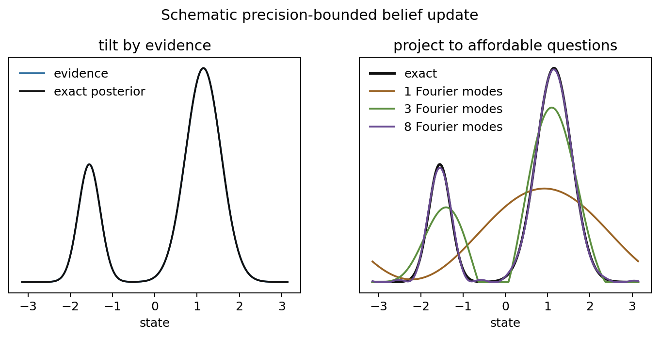
Figure 1. A schematic bounded update. Exact evidence produces a posterior with fine structure. Projection to a small number of modes preserves only the distinctions available to the bounded question space.

5. A Worked Example on the Circle

Let (X=S^1), parameterized by (x\in[-\pi,\pi]). Take the Fourier basis

\[1,\ \cos x,\ \sin x,\ \cos 2x,\ \sin 2x,\ldots\]

and define (\mathcal Q_r) to be the span of modes up to frequency (r). Let (\Pi_r) be (L^2) projection onto (\mathcal Q_r). If a prior density (p(x)) is updated by likelihood (\ell(x)), the exact posterior is

\[p^\ell(x)=\frac{\ell(x)p(x)}{\int \ell p}.\]

The bounded posterior is represented only through the low-frequency expectations

\[b_r^\ell(q)= \frac{\int \Pi_r(q\ell)(x)p(x)\,dx} {\int \Pi_r(\ell)(x)p(x)\,dx}, \qquad q\in\mathcal Q_r.\]

If (\ell) has narrow spikes, the exact posterior contains high-frequency structure. Small (r) erases it. Increasing (r) restores it.

Proposition 2. Suppose (p,\ell,q\in L^2(S^1)), (\ell\ge 0), and (\int \ell p>0). If (\Pi_r\to I) strongly in (L^2), then for every bounded (q) with (q\ell\in L^2),

\[b_r^\ell(q)\to b^\ell(q),\]

provided the denominators remain bounded away from zero.

Proof. Strong convergence gives

\[\|\Pi_r(q\ell)-q\ell\|_{L^2}\to 0\]

and

\[\|\Pi_r(\ell)-\ell\|_{L^2}\to 0.\]

Pairing with (p\in L^2) is continuous by Cauchy-Schwarz, so the numerator and denominator converge to their exact values. If the denominator stays bounded away from zero, the quotient converges. (\square)

This is the clean sense in which bounded Bayes approaches ordinary Bayes as the representable question space grows.

6. Error Accounting

The capacity framework from Part I supplies approximation targets. Let (T) be an exact whitened update or transport operator, and let (T_r) be its best rank-(r) approximation. If

\[s_1\ge s_2\ge \cdots\]

are the singular values of (T), then the Eckart-Young-Mirsky theorem gives

\[\|T-T_r\|_{\mathrm{op}}=s_{r+1},\]

and

\[\|T-T_r\|_{\mathrm{HS}}^2=\sum_{i>r}s_i^2.\]

For a capacity functional of the form

\[C_\alpha(T)=\frac12\sum_i\log(1+\alpha s_i^2),\]

the discarded capacity satisfies

\[0\le C_\alpha(T)-C_\alpha(T_r) = \frac12\sum_{i>r}\log(1+\alpha s_i^2).\]

Thus a bounded update has several separable error sources:

1. approximation error from using the wrong question family;
2. spectral truncation error from finite rank or finite capacity;
3. sample error from estimating operators;
4. positivity error from projection;
5. normalization error from estimating evidence probability.

The benefit of the operator picture is that these errors can be assigned to different steps.

7. Sequential Bounded Updates

Suppose an exact computation is a product of update operators:

\[T=T_mT_{m-1}\cdots T_1.\]

Let (\widetilde T_i) be bounded approximations. If all later exact operators and approximations are contractions in the same norm, then local errors add:

\[\|T-\widetilde T\| \le \sum_{i=1}^m\|T_i-\widetilde T_i\|.\]

Proof. Use the telescoping identity

\[T_m\cdots T_1-\widetilde T_m\cdots \widetilde T_1 = \sum_{i=1}^m T_m\cdots T_{i+1}(T_i-\widetilde T_i) \widetilde T_{i-1}\cdots \widetilde T_1.\]

Taking norms and using contractivity of every surrounding factor gives the bound. (\square)

This is not a free stability theorem. The contraction assumption is substantive. It says the noise/energy geometry is aligned with the update process strongly enough that compression errors do not amplify.

8. Order Effects from Projection

Exact classical evidence multiplication commutes:

\[M_{\ell_1}M_{\ell_2}=M_{\ell_2}M_{\ell_1}.\]

Projected updates need not commute:

\[\Pi_BM_{\ell_1}\Pi_BM_{\ell_2}\Pi_B \ne \Pi_BM_{\ell_2}\Pi_BM_{\ell_1}\Pi_B.\]

This is a bounded-computation effect. The underlying evidence functions still commute. The order dependence comes from throwing away different components after the first update.

Proposition 3. Compressed evidence updates need not commute.

Proof. The commutator

\[[\Pi_BM_{\ell_1}\Pi_B,\Pi_BM_{\ell_2}\Pi_B]\]

is not identically zero. Here is a finite example. Let (X={1,2,3}), let multiplication by evidence be diagonal in the point basis, and project onto the two-dimensional subspace with orthonormal basis

\[q_1=\frac{(1,1,1)}{\sqrt 3}, \qquad q_2=\frac{(1,-1,0)}{\sqrt 2}.\]

Take

\[M_{\ell_1}=\operatorname{diag}(1,2,4), \qquad M_{\ell_2}=\operatorname{diag}(2,5,7).\]

In the ((q_1,q_2)) basis, the compressed operators (\Pi_BM_{\ell_i}\Pi_B) have matrices

\[A= \begin{pmatrix} 7/3 & -1/\sqrt 6\\ -1/\sqrt 6 & 3/2 \end{pmatrix}, \qquad B= \begin{pmatrix} 14/3 & -3/\sqrt 6\\ -3/\sqrt 6 & 7/2 \end{pmatrix}.\]

Their commutator has off-diagonal entry

\[[A,B]_{12} = -\frac{4}{3\sqrt 6}\ne 0.\]

Thus the compressed updates do not commute, even though the original multiplication operators do. (\square)

This resembles quantum order effects at the level of update algebra, but the source is different. Quantum probability starts with noncommutative observables. Bounded RKHS Bayes starts with classical functions and introduces noncommutativity through compression. Treating these as identical would be a category error.

9. What This Does and Does Not Claim

This framework does not say that agents literally store RKHS elements. It defines a mathematical object for representing finite-precision access to a state space.

It also does not say that every projection is normatively correct. The projection is part of the model. Different kernels, budgets, and positivity constraints define different bounded agents.

The claim is narrower: once the affordable question space is specified, belief updates can be written as observable updates, and their approximation error can be studied spectrally.

10. Summary

Part I treated functions as signals. Part II treats beliefs as bounded answer functionals over those functions.

The exact Bayesian formula

\[b^\ell(q)=\frac{b(\ell q)}{b(\ell)}\]

becomes bounded Bayes by inserting a projection:

\[b_B^\ell(q) = \frac{b(\Pi_B(q\ell))} {b(\Pi_B(\ell))}.\]

At infinite capacity this approaches classical Bayes. At finite capacity it becomes a controlled approximation with spectral, sampling, positivity, and normalization errors.

Part III applies the same operator viewpoint to computations. A hidden state will be treated as a mediator between past and future, or between input and behavioral output, and the question becomes which modes are associated through that mediator.

References

• Kolmogorov, A. N. Foundations of the Theory of Probability. 1933.
• Jaynes, E. T. Probability Theory: The Logic of Science. Cambridge University Press, 2003.
• Aronszajn, N. “Theory of Reproducing Kernels.” Transactions of the American Mathematical Society, 1950.
• Fukumizu, K., Song, L., and Gretton, A. “Kernel Bayes’ Rule.” arXiv:1009.5736, https://arxiv.org/abs/1009.5736.
• Song, L., Fukumizu, K., and Gretton, A. “Kernel Embeddings of Conditional Distributions.” IEEE Signal Processing Magazine, 2013.
• Muandet, K., Fukumizu, K., Sriperumbudur, B., and Schölkopf, B. “Kernel Mean Embedding of Distributions: A Review and Beyond.” arXiv:1605.09522, https://arxiv.org/abs/1605.09522.
• Nielsen, M. A. and Chuang, I. L. Quantum Computation and Quantum Information. Cambridge University Press, 2010.
• Bhatia, R. Matrix Analysis. Springer, 1997.

LLM Usage

The source conversation for Parts I and II was https://chatgpt.com/share/6a4bdbee-c8d8-83eb-a58d-38b213087b2f. This post was written with assistance from GPT5.5-Pro and Codex. Any errors are my responsibility.