[AI-Written] Information in Continua III: Sequential Computations

Author’s note. This three-part series is a writeup of a kernel-based analogue of information theory I have been developing over the course of my research at MATS and the Iliad Fellowship. It has taken on enough substantive form that I’m pleased to share it. The motivation is to develop an analogue of information theory which is better suited to the description of continuous spaces and computations thereon. This permits a native notion of ‘resolution’ and ‘imprecision’. The particular problem I wanted to resolve is that, for a function $f(x)$, we can only measure it at finite resolution, so fluctuations on unresolved scales could in principle carry large amounts of information, and to do this in a way that permits treating these fluctuations and noise on a distinct footing. Because of this resolution-centered perspective, I expect the theory to be useful for probing information in functions, as the objects are well-suited for spectral approximation.

The theory starts by developing a function-space analogue of channel-capacity in part I, extends this to a notion of resolution-bounded probability in part II, and in part III develops an application to continuous-space computations.

I decided to have GPT5.5-Pro write these up, judging that it was less likely to make mistakes than me. I apologize in advance for any cringe.

Research context. This work was developed during MATS 9.1 under Richard Ngo and during the Iliad Fellowship under Dmitry Vaintrob.

1. Hidden States as Mediators

Parts I and II developed information and belief in terms of affordable observable functions. Part III applies the same idea to computation.

The target is a factored computation

\[X \xrightarrow{\psi} H \xrightarrow{\varphi} Y.\]

Here $X$ is the input or past, $H$ is an intermediate state, and $Y$ is the output or future. The state $H$ is not assigned meaning by its coordinates. It is assigned a mathematical role: it mediates a factorization from $X$ to $Y$.

The interpretability question is therefore not merely:

\[\text{Can I decode feature } f \text{ from } H?\]

but:

\[\text{Which input distinctions are associated through } H \text{ with output distinctions?}\]

This framing does not make modes semantic by decree. The user chooses $X,H,Y$, kernels, and behavioral observables. The theory then returns spectral objects for that specified experiment.

2. Conditional Mean Embedding Operators

Choose kernels $k_X,k_H,k_Y$ and RKHSs $\mathcal H_X,\mathcal H_H,\mathcal H_Y$. Let $\Phi_X,\Phi_H,\Phi_Y$ be the feature maps. I use the convention

\[(a\otimes b)f=a\,\langle b,f\rangle,\]

so $a\otimes b$ maps from the Hilbert space containing $b$ to the Hilbert space containing $a$.

For random variables $A,B$, write

\[C_{BA} = \mathbb E\left[(\Phi_B(B)-\mu_B)\otimes(\Phi_A(A)-\mu_A)\right]\]

for the centered cross-covariance operator. The centered conditional mean embedding, or equivalently the RKHS regression operator, is

\[U_{B\mid A}=C_{BA}C_{AA}^{\dagger}:\mathcal H_A\to\mathcal H_B,\]

with Moore-Penrose inverse on the relevant closed range. In finite samples one uses the ridge version

\[U_{B\mid A}^{\lambda}=C_{BA}(C_{AA}+\lambda I)^{-1}.\]

The adjoint $U_{B\mid A}^*$ sends an observable $g\in\mathcal H_B$ to the RKHS projection of the conditional expectation

\[a\mapsto \mathbb E[g(B)-\mathbb E g(B)\mid A=a].\]

With uncentered covariances, or with constants explicitly included in the RKHS, the same construction gives the usual conditional mean embedding $a\mapsto\mu_{B\mid a}$. I use the centered version because the routing object concerns fluctuations and distinctions around the mean, not the unconditional mean component.

For the factored computation $X\to H\to Y$, define the encoder and decoder conditional operators

\[U_{H\mid X}=C_{HX}C_{XX}^{\dagger}, \qquad U_{Y\mid H}=C_{YH}C_{HH}^{\dagger}.\]

The mediated conditional operator through the chosen state $H$ is

\[U^{(H)}_{Y\mid X} = U_{Y\mid H}U_{H\mid X}.\]

This is the primary object. It says: take an $X$-side distinction, map it to the conditional mean hidden-state distinction, then map that hidden-state distinction to the conditional mean output distinction.

The spectral calculations below use covariance-normalized coordinates for these CMEs. Define

\[T_{H\mid X} = C_{HH}^{-1/2}C_{HX}C_{XX}^{-1/2}.\]

Equivalently,

\[T_{H\mid X}=C_{HH}^{-1/2}U_{H\mid X}C_{XX}^{1/2}.\]

Likewise

\[T_{Y\mid H}=C_{YY}^{-1/2}U_{Y\mid H}C_{HH}^{1/2} =C_{YY}^{-1/2}C_{YH}C_{HH}^{-1/2}.\]

These are whitened representations of conditional mean embedding operators. Their singular values are kernel canonical correlations. They describe which normalized function-space modes of one variable predict normalized function-space modes of another.

The use of kernels matters for the same reason it mattered in Part I. $L^2$ over all measurable functions is too large for many deterministic computations: pullbacks can become isometries and thereby erase the distinction between smooth structure and microscopic coding. The kernel restricts the question class.

3. CME Factorization Through a State

For a deterministic split $Y=\varphi(H)$, and more generally for a stochastic mediator, the relevant conditional-independence condition is

\[X\perp Y\mid H\]

relative to the joint distribution being studied. This statement does not by itself make arbitrary centered covariance operators multiply exactly. The clean statement is about conditional mean embedding operators, and it needs the usual range and closure assumptions: the conditional expectations being represented should lie in the chosen RKHSs, or should be read after projection into them.

Proposition 1. Suppose $X\perp Y\mid H$, the relevant centered CMEs exist, and for every $g\in\mathcal H_Y$ the conditional expectations below are represented in the chosen RKHSs. Then

\[U_{Y\mid X} = U_{Y\mid H}U_{H\mid X}.\]

Proof. It is enough to compare adjoints on observables $g\in\mathcal H_Y$. By the defining property of the centered CME adjoint,

\[(U_{Y\mid X}^*g)(X) = \mathbb E[g(Y)-\mathbb E g(Y)\mid X].\]

Using $X\perp Y\mid H$ and the tower property,

\[\mathbb E[g(Y)-\mathbb E g(Y)\mid X] = \mathbb E\left[ \mathbb E[g(Y)-\mathbb E g(Y)\mid H]\mid X \right].\]

The inner conditional expectation is represented by the adjoint decoder. Applying the defining property of the adjoint encoder gives

\[(U_{Y\mid X}^*g)(X) = (U_{H\mid X}^*U_{Y\mid H}^*g)(X).\]

Thus

\[U_{Y\mid X}^*=U_{H\mid X}^*U_{Y\mid H}^*,\]

and therefore

\[U_{Y\mid X}=U_{Y\mid H}U_{H\mid X}.\]

(\square)

In the covariance-normalized coordinates, the direct $X$-to-$Y$ conditional operator is

\[T_{Y\mid X} = C_{YY}^{-1/2}U_{Y\mid X}C_{XX}^{1/2}.\]

The mediated version is

\[T^{(H)}_{Y\mid X} = C_{YY}^{-1/2}U_{Y\mid H}U_{H\mid X}C_{XX}^{1/2}.\]

Using the definitions above,

\[T^{(H)}_{Y\mid X} = T_{Y\mid H}T_{H\mid X}.\]

For finite samples, the regularized estimator is

\[U^{(H;\lambda_H,\lambda_X)}_{Y\mid X} = C_{YH}(C_{HH}+\lambda_H I)^{-1} C_{HX}(C_{XX}+\lambda_X I)^{-1}.\]

This should be read as a ridge-CME approximation to the mediated conditional operator, not as an exact identity. If a residual or skip path bypasses $H$, or if the conditional-embedding assumptions fail, the mediated conditional operator describes only the dependence explained by the chosen state. The residual

\[T_{Y\mid X}-T^{(H)}_{Y\mid X}\]

is then evidence that the chosen state is not a complete mediator in the chosen RKHS geometry.

4. The Routing Matrix

Take singular value decompositions:

\[T_{H\mid X} = \sum_j \sigma_j\, w_j\otimes u_j,\]

where $u_j\in\mathcal H_X$, $w_j\in\mathcal H_H$, and $\sigma_j$ is the encoder strength. Similarly,

\[T_{Y\mid H} = \sum_k \tau_k\, v_k\otimes \widetilde w_k,\]

where $\widetilde w_k\in\mathcal H_H$, $v_k\in\mathcal H_Y$, and $\tau_k$ is the decoder strength.

The encoder gives hidden modes associated with the input. The decoder gives hidden modes associated with the output. Since both hidden-mode systems live in $\mathcal H_H$, define

\[R_{jk}=\langle \widetilde w_k,w_j\rangle_{\mathcal H_H}.\]

This is the routing matrix.

Proposition 2. Under the CME factorization above,

\[T^{(H)}_{Y\mid X} = \sum_{j,k}\sigma_j R_{jk}\tau_k\, v_k\otimes u_j.\]

Proof. Compose the two SVD expansions:

\[T_{Y\mid H}T_{H\mid X} = \sum_{j,k} \sigma_j\tau_k (v_k\otimes \widetilde w_k)(w_j\otimes u_j).\]

For rank-one operators,

\[(v\otimes \widetilde w)(w\otimes u) = \langle \widetilde w,w\rangle v\otimes u.\]

Therefore

\[T_{Y\mid H}T_{H\mid X} = \sum_{j,k}\sigma_j \langle \widetilde w_k,w_j\rangle_{\mathcal H_H} \tau_k\,v_k\otimes u_j.\]

Using Proposition 1 gives the result. $\square$

The interpretation is literal and limited:

• $\sigma_j$ measures how strongly input mode $j$ is associated with the hidden state;
• $R_{jk}$ measures how much that hidden mode overlaps an output-relevant hidden mode;
• $\tau_k$ measures how strongly output mode $k$ is observed from the hidden state.

Thus the product $\sigma_jR_{jk}\tau_k$ is a modewise contribution to the whitened mediated CME.

5. Gauge Invariance

Hidden coordinates are not canonical. A rotation, translation, or other kernel-preserving reparameterization of $H$ should not change the routing description.

Call a reparameterization $\Gamma:H\to H$ kernel-isometric if

\[k_H(\Gamma(h),\Gamma(h'))=k_H(h,h')\]

for all $h,h’$. It induces a unitary operator $U_\Gamma$ on $\mathcal H_H$.

Proposition 3. When the relevant singular values are nondegenerate and signs/phases are fixed consistently, the routing entries are invariant under kernel-isometric reparameterizations. In degenerate singular subspaces, the invariant object is the block or subspace routing map, not individual entries.

Proof. Under the reparameterization, encoder hidden modes transform as $w_j\mapsto U_\Gamma w_j$, and decoder hidden modes transform as $\widetilde w_k\mapsto U_\Gamma\widetilde w_k$. For a nondegenerate singular value, the corresponding singular vector is unique up to sign or phase; fix this convention consistently. Since $U_\Gamma$ is unitary,

\[R'_{jk} = \langle U_\Gamma\widetilde w_k,U_\Gamma w_j\rangle_{\mathcal H_H} = \langle \widetilde w_k,w_j\rangle_{\mathcal H_H} = R_{jk}.\]

$\square$

The qualifier matters twice. The routing matrix is not invariant to arbitrary changes of geometry. If the kernel changes, the question changes. And when singular values are repeated, rotations inside the degenerate singular subspace change the displayed entries of $R$; then only the associated subspaces, principal angles, or block norms should be interpreted.

6. Sequential Computations and Hankel Structure

For sequential systems, $X$ can be the past and $Y$ the future:

\[X_t=(\ldots,u_{t-2},u_{t-1}),\qquad Y_t=(y_t,y_{t+1},\ldots).\]

The classical Hankel operator maps pasts to futures. Its singular values are the Hankel singular values of the system. In linear systems theory, balanced realization keeps the directions that are both reachable from inputs and observable in outputs. The present construction is a kernelized diagnostic inspired by that picture:

• encoder modes are past-to-state predictive modes;
• decoder modes are state-to-future predictive modes;
• the routing matrix measures how the two hidden geometries overlap.

This is why sequential computation is the cleanest case. Past-future structure supplies a canonical source of observables. In deterministic dynamical systems, delay coordinates and Koopman-style observable families are natural. In single-pass feedforward networks, there is no automatic delay construction, so the kernel choice carries more modeling weight.

7. Worked Example: Same Function, Different Algorithm

Consider two finite-state transducers computing binary increment:

\[0110\mapsto 0111,\qquad 0111\mapsto 1000.\]

System A scans from the least significant bit, propagating a carry until it finds a zero. System B first scans to mark the rightmost zero, then performs a second pass to flip the suffix.

The input-output function is the same. The internal computation is not.

Let $H^{(t)}$ be the configuration at time $t$: finite control state, head position, and tape contents. Use a Hamming kernel on binary strings,

\[k(s,s')=\exp(-d_{\mathrm{Ham}}(s,s')/\alpha),\]

and a one-hot kernel on finite control states. At each time $t$, compute a routing matrix

\[R^{(t)}_{jk} = \langle \widetilde w_k^{(t)},w_j^{(t)}\rangle_{\mathcal H_{H^{(t)}}}.\]

For the carry-propagation algorithm, the mediated associations are local: the bits already scanned are the bits whose outputs have been determined. The routing matrix is close to diagonal. For the two-pass algorithm, the first pass associates many inputs with a summary-like state without yet associating them with the corresponding output distinctions; the second pass associates outputs with that summary. The routing pattern changes over time.

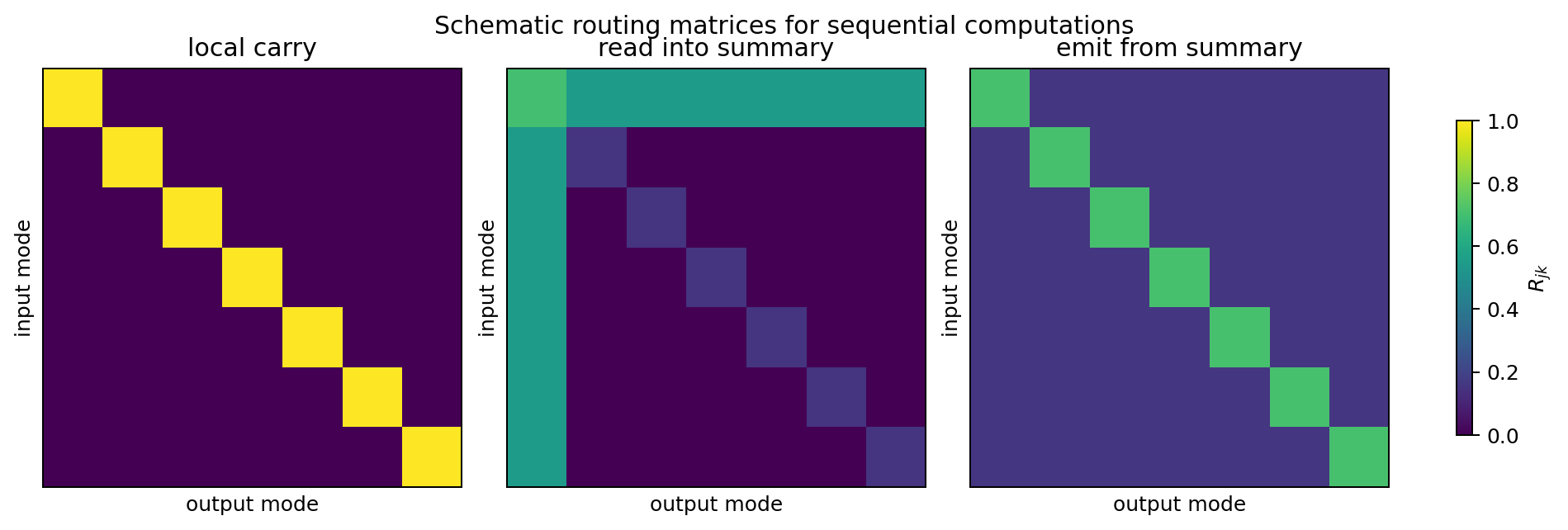
Figure 1. Schematic routing matrices. A local carry algorithm associates input modes with corresponding output modes through the current state. A two-pass algorithm first associates many inputs with a summary-like direction, then later associates output distinctions with it. These panels are illustrative, not empirical measurements.

The point is not that these heatmaps are the final algorithmic metric. The point is that the object being compared is no longer only the end-to-end function. It is the sequence

\[\left((\sigma^{(t)},R^{(t)},\tau^{(t)})\right)_{t=1}^T.\]

This sequence can differ even when the input-output map is identical.

8. Estimation

In finite data, estimate the ridge CMEs and then take the SVD of their covariance-normalized representations. Equivalently, compute kernel CCA/SVD on the $(X,H)$ and $(H,Y)$ pairs.

1. Build Gram matrices $G^X,G^H,G^Y$.
2. Center and regularize them.
3. Compute CCA/SVD for $(X,H)$ and $(H,Y)$.
4. Represent hidden CCA modes by coefficient vectors.
5. Compute empirical routing entries by RKHS inner products:

\[\widehat R_{jk} = (\widehat\alpha^{HX}_j)^\top G^H\widehat\alpha^{YH}_k,\]

with cosine normalization if regularization changes the empirical mode norms.

The fundamental reliability condition is spectral separation. If $\sigma_j\approx\sigma_{j+1}$, the individual modes are unstable, though their span may still be meaningful.

By Wedin-style singular subspace perturbation bounds,

\[\sin\angle(\widehat u_j,u_j) \lesssim \frac{\|\widehat C-C\|_{\mathrm{op}}} {\operatorname{gap}_j}.\]

Here $\operatorname{gap}_j$ is the relevant separation between the singular value or singular-value cluster being estimated and the rest of the spectrum. Closely spaced modes require larger samples, and routing entries involving them should not be overinterpreted. Stable block structure is safer than individual entries.

9. Relation to Probes

A probe asks whether a feature is decodable from $H$. A routing decomposition asks whether an input-side mode changes the conditional mean embedding of the output through $H$, and which output-side modes receive that change.

These are different questions. A feature can be present while having little mediated association with the chosen output observable. A feature can matter for one behavioral observable $Y$ and be irrelevant for another. Changing $Y$ changes the decoder and therefore changes $R$.

Examples of possible $Y$’s include logits, labels, reward-model scores, refusal indicators, or any other specified behavioral target. The theory does not say these observables are intrinsically important. It says that once $Y$ is specified, the factorization can be decomposed relative to it.

10. Limitations

Kernel dependence. The routing matrix is relative to $k_X,k_H,k_Y$. Different kernels ask different questions. Cross-kernel comparison should emphasize persistent spectral features, not entrywise equality.

Incomplete mediation. Residual streams and skip connections can violate $X\perp Y\mid H$. Then the mediated conditional operator through $H$ describes only the dependence explained by the chosen slice, not the whole computation.

No automatic semantics. Modes are function-space directions. Human interpretation requires further empirical work, such as examples, interventions, or controlled datasets.

Sample complexity. Kernel methods can be expensive. Nyström approximations, random Fourier features, and randomized SVD are practical options, but they introduce approximation error.

LLM status. The framework is a proposed measurement language and has toy examples. It is not yet evidence that a production language model uses a particular human-legible algorithm.

11. Summary

The three posts now form a single chain.

Part I: information is capacity over distinguishable low-energy functions.

Part II: belief is a bounded ability to answer affordable questions.

Part III: computation composes conditional mean embedding operators through intermediate states.

The main conditional operator is

\[U^{(H)}_{Y\mid X} = U_{Y\mid H}U_{H\mid X}.\]

After covariance normalization, its spectral coordinate representation is

\[T^{(H)}_{Y\mid X} = T_{Y\mid H}T_{H\mid X}.\]

The central finite-dimensional summary is

\[R_{jk} = \langle \widetilde w_k,w_j\rangle_{\mathcal H_H},\]

where $w_j$ is a hidden mode associated with the input and $\widetilde w_k$ is a hidden mode associated with the output. Together with $\sigma_j$ and $\tau_k$, it decomposes the whitened mediated CME into spectral channels:

\[T^{(H)}_{Y\mid X} = \sum_{j,k}\sigma_jR_{jk}\tau_k\,v_k\otimes u_j.\]

That is the continuous-space analogue of asking which parts of the state are jointly input-predictive, output-predictive, and aligned in the chosen hidden-state geometry.

References

• Ho, B. L. and Kalman, R. E. “Effective Construction of Linear State-Variable Models from Input/Output Functions.” Regelungstechnik, 1966.
• Fliess, M. “Matrices de Hankel.” Journal de Mathématiques Pures et Appliquées, 1974.
• Van Overschee, P. and De Moor, B. Subspace Identification for Linear Systems. Kluwer, 1996.
• Takens, F. “Detecting Strange Attractors in Turbulence.” In Dynamical Systems and Turbulence, Lecture Notes in Mathematics 898, 1981.
• Koopman, B. O. “Hamiltonian Systems and Transformation in Hilbert Space.” Proceedings of the National Academy of Sciences, 1931.
• Bach, F. R. and Jordan, M. I. “Kernel Independent Component Analysis.” Journal of Machine Learning Research, 2002.
• Fukumizu, K., Song, L., and Gretton, A. “Kernel Bayes’ Rule.” arXiv:1009.5736, https://arxiv.org/abs/1009.5736.
• Song, L., Fukumizu, K., and Gretton, A. “Kernel Embeddings of Conditional Distributions.” IEEE Signal Processing Magazine, 2013.
• Wedin, P. A. “Perturbation Bounds in Connection with Singular Value Decomposition.” BIT Numerical Mathematics, 1972.
• Rahimi, A. and Recht, B. “Random Features for Large-Scale Kernel Machines.” NeurIPS, 2007.
• Halko, N., Martinsson, P. G., and Tropp, J. A. “Finding Structure with Randomness: Probabilistic Algorithms for Constructing Approximate Matrix Decompositions.” arXiv:0909.4061, https://arxiv.org/abs/0909.4061.

LLM Usage

This post was written with assistance from GPT5.5-Pro and Codex. I do not have the source chats for Part III; it was based on local notes and drafts, especially the spectral-state/routing-matrix material. Any errors are my responsibility.