Data attribution · Lecture 2

Curvature at scale

From Hessian-vector products to the spectrum of a 100B-parameter model

Where we are

This morning gave the formula

$$\mathcal I_i=-\nabla\phi^\top(G+\lambda I)^{-1}\nabla L_i$$

For a 1B-parameter model, the matrix inside has $10^{18}$ entries.

The plan

Three questions need only products $v\mapsto Hv$

$v\ \mapsto\ Hv$

→

solve $(H+\lambda I)x=g$

→

top eigenpairs

→

spectral density $\rho(s)$: where the eigenvalues sit

$H$: the $P\times P$ Hessian of the training loss (or $G$, its Gauss–Newton part).

§1 · The primitive

How do you multiply by a Jacobian you can't even store?

§1 · Two directions

Forward and reverse mode

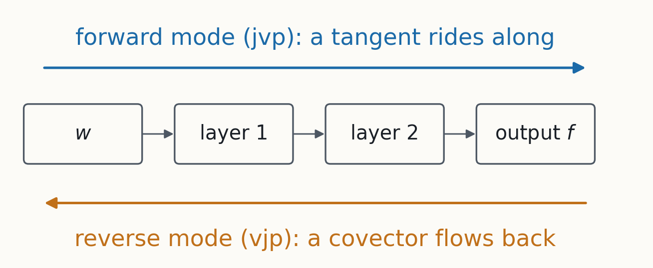
A chain of layers; forward mode carries a tangent left to right, reverse mode carries a covector right to left

Forward mode pushes a tangent through; reverse mode pulls a covector back.

§1 · The two products

jvp and vjp, for a Jacobian $J$

$$\underbrace{v\mapsto Jv}_{\text{jvp}}\qquad\htmlClass{fragment}{\underbrace{u\mapsto J^\top u}_{\text{vjp}}}$$

Each costs a few forward passes, at any size; backprop is a vjp.

§1 · A tiny example

Forward mode is arithmetic with dual numbers

$$\begin{aligned} &f(x_1,x_2)=x_1x_2+\sin x_1,\qquad x_1=1+\varepsilon,\ \ x_2=2,\ \ \varepsilon^2=0\\[6pt] &\htmlClass{fragment}{f=(2+\sin 1)+(2+\cos 1)\,\varepsilon} \end{aligned}$$

The $\varepsilon$-coefficient is $\partial f/\partial x_1$: a jvp with $v=(1,0)$.

§1 · From gradients to Hv

Move along $v$ and watch the gradient

$$\nabla L(w+rv)=\nabla L(w)+r\,Hv+O(r^2)$$

The gradient changes along $v$ at rate $Hv$.

§1 · From gradients to Hv

So $Hv$ is a directional derivative of the gradient

$$Hv=\frac{d}{dr}\,\nabla L(w+rv)\Big|_{r=0}$$

And a directional derivative is exactly what a jvp computes.

§1 · Pearlmutter's trick

$Hv$ is a jvp of the gradient function

$$Hv=\operatorname{jvp}\big(\nabla L;\ w,\ v\big)\qquad\htmlClass{fragment}{=\ \nabla_w\big(\nabla L^\top v\big)}$$

Exact, for about two to three gradients' worth of work.

§1 · Gauss–Newton

The Gauss–Newton product, piece by piece

$$Gv=\sum_i\ \underbrace{J_i^\top}_{\text{vjp}}\ \underbrace{H_{y,i}}_{\substack{\text{loss Hessian}\\ \text{in the outputs}}}\ \underbrace{(J_iv)}_{\text{jvp}}$$

$J_i$: the Jacobian of the outputs on example $i$. One jvp, a small multiply, one vjp.

§1 · Without double differentiation

Or just take two ordinary gradients

$$Hv\approx\frac{\nabla L(w+\epsilon v)-\nabla L(w-\epsilon v)}{2\epsilon}$$

Works inside any training loop. But which $\epsilon$?

§1 · Two errors

Truncation versus round-off

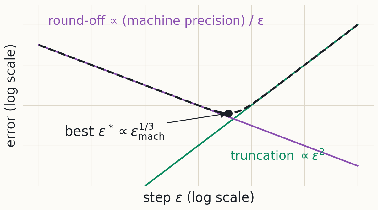
Schematic: truncation error grows like epsilon squared, round-off like one over epsilon; their sum has a minimum

Shrink $\epsilon$ and round-off grows; enlarge it and truncation grows.

Granziol & Juarev (2026), Thm 3.1, for unit $v$: error $\le\frac{\epsilon^2}{6}\|\nabla_w(D_v^3L)\|+O(\frac{\epsilon_{\rm mach}}{\epsilon}\|\nabla L\|)$, with $D_v^3L$ the third derivative of $L$ along $v$. Leading order; a rigorous version takes the sup of that fourth derivative over the segment. Balancing gives $\epsilon^*\propto\epsilon_{\rm mach}^{1/3}$ and best error $\propto\epsilon_{\rm mach}^{2/3}$.

Their Remark 3.2: fp32 $\epsilon^*\sim10^{-3}$–$10^{-2}$, errors $\sim10^{-5}$; bf16 $\epsilon^*\sim10^{-1}$, errors $\sim10^{-2}$.

Identity: the gradient central difference is exactly the average of $H(w+tv)v$ over $t\in[-\epsilon,\epsilon]$. A large $\epsilon$ gives curvature averaged along a segment, not a noisy $Hv$. (Their Thm 3.3 is the triangular-kernel version for the second difference of $L$.)

§1 · Measured

On a real network you get the V

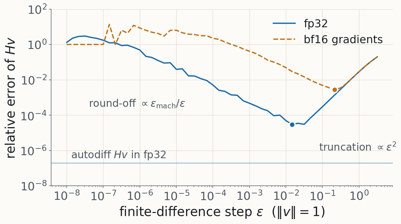
Relative error of the finite-difference Hv against autodiff Hv as a function of epsilon, in fp64, fp32 and with bf16-rounded gradients

The best $\epsilon$ moves with precision: sweep it against an exact $Hv$.

§1 · Takeaway

$Hv$ costs a few gradients: exact by autodiff, or two gradients and a well-chosen $\epsilon$.

§2 · What products buy

You have a function that returns $Hv$. What can you compute with it?

§2 · Hutchinson

A trace from ten products

$$\operatorname{tr}H=\mathbb E_v\big[v^\top Hv\big]\quad\text{for }\mathbb E[vv^\top]=I$$

Hutchinson: random $\pm1$ probes $v$, one $Hv$ each.

§2 · Solves

Solves are the expensive question

An IF needs one solve per query.
Iterative solvers can need thousands of $Hv$ per solve.
That cost is why DA2 uses EK-FAC for IFs.

§2 · Eigenvalues

How do you find the top eigenvalues from $Hv$ alone?

§2 · Krylov

Repeated multiplication tilts $v$ toward the top

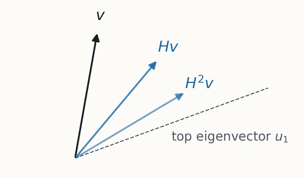
Unit vectors v, Hv, H squared v rotating toward the top eigenvector of a 2 by 2 matrix

Keep all of $v, Hv, H^2v,\dots$: their span is the Krylov subspace.

§2 · Lanczos

$m$ products compress $H$ to a tridiagonal matrix

$$T_m=Q_m^\top H Q_m=\begin{pmatrix}\alpha_1&\beta_1&\\ \beta_1&\alpha_2&\ddots\\ &\ddots&\ddots\end{pmatrix}$$

$H$ restricted to the Krylov basis $Q_m$; its eigenvalues, the Ritz values $\theta_k$, approximate $H$'s.

§2 · A 4×4 example

A 4×4 example: watch the Ritz values

$$\begin{aligned} m=1:&\quad 0.55\\ \htmlClass{fragment}{m=2:}&\quad\htmlClass{fragment}{0.30,\ \ 4.82}\\ \htmlClass{fragment}{m=3:}&\quad\htmlClass{fragment}{0.23,\ \ 0.81,\ \ 5.00}\\ \htmlClass{fragment}{m=4:}&\quad\htmlClass{fragment}{0.2,\ \ 0.5,\ \ 1,\ \ 5} \end{aligned}$$

True eigenvalues $0.2,\ 0.5,\ 1,\ 5$: the extremes arrive first.

§2 · On a network

Outliers converge fast; the bulk is slow

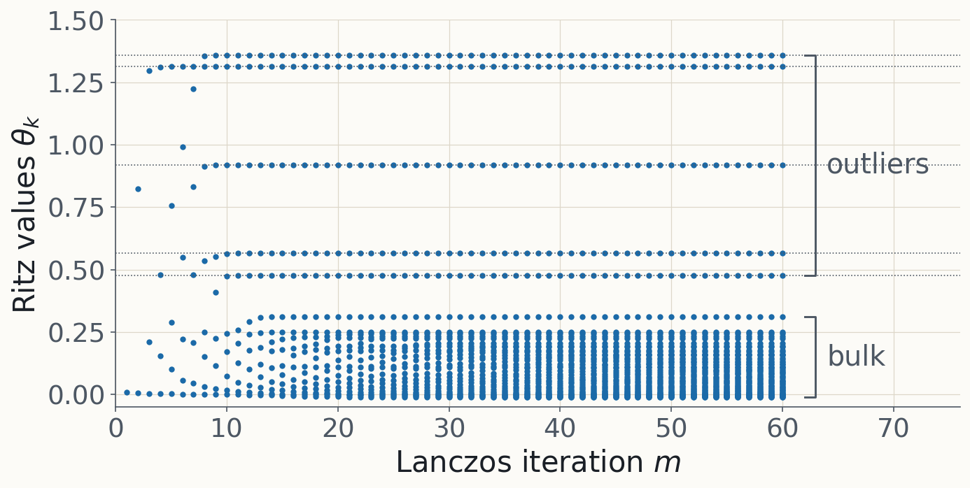
Ritz values against Lanczos iteration with full reorthogonalization

Toy MLP: the five outliers are done by about $m=12$.

§2 · Floating point

Without reorthogonalization: ghosts

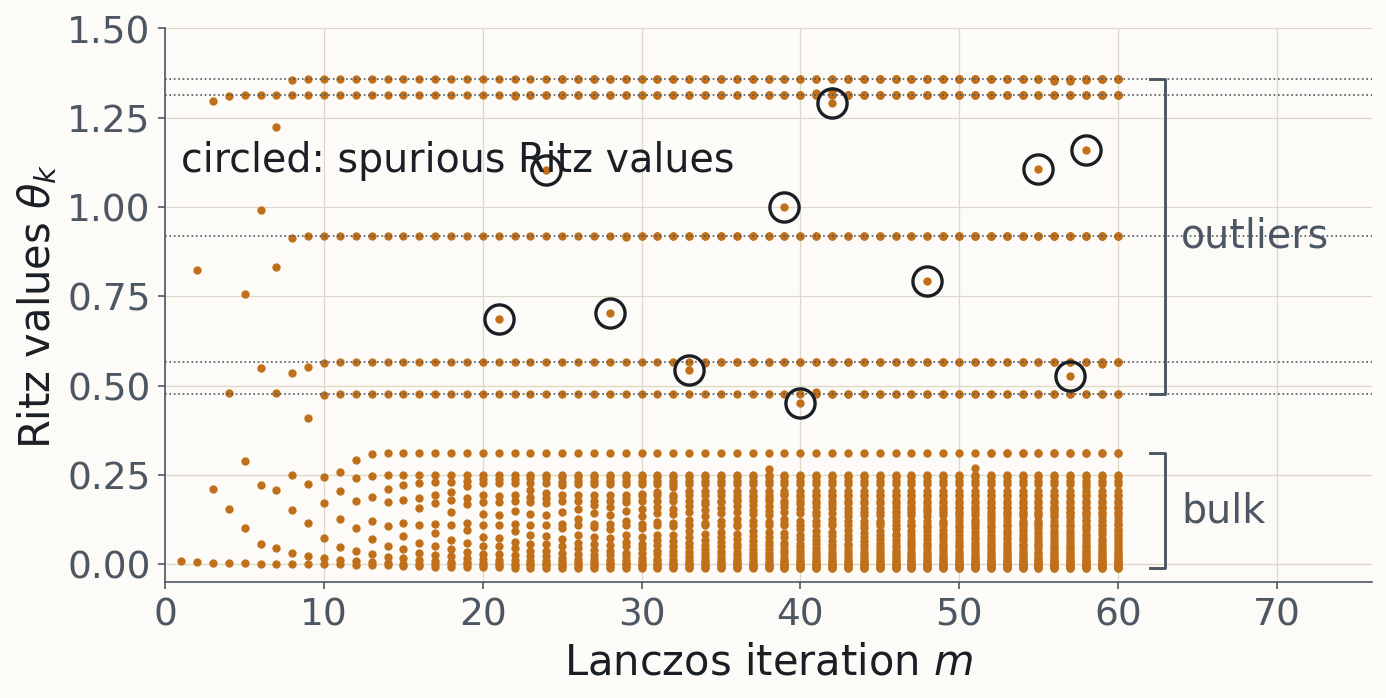
Ritz values against Lanczos iteration without reorthogonalization, showing spurious copies

Lost orthogonality creates spurious Ritz values and copies of converged ones.

§2 · The memory wall

Reorthogonalizing needs every basis vector

$$\text{one vector}=P\ \text{numbers}:\quad P=10^{11}\ \text{in bf16}\ \Rightarrow\ 200\ \text{GB}$$

Keeping $m$ of them is out of reach at LLM scale, so $m$ stays small.

§2 · Takeaway

Lanczos finds the outliers in a few steps; the bulk stays a blur.

§3 · The whole spectrum

Lanczos found the outliers. Can the same $T_m$ give the whole spectrum?

§3 · Step 1

What a single probe sees

$$v^\top f(H)\,v=\sum_j\,(v\cdot u_j)^2\,f(\lambda_j)$$

Each eigenvalue, weighted by the probe's overlap with its eigenvector.

§3 · Step 2

That sum is an integral against sticks

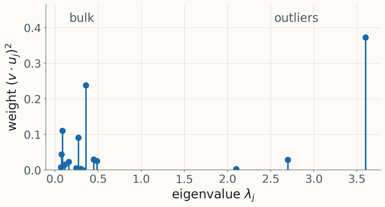
Eigenvalue sticks whose heights are the probe weights

$v^\top f(H)v=\int f\,d\mu_v$: a stick at each $\lambda_j$, height $(v\cdot u_j)^2$.

§3 · Step 3

Lanczos gives the Gauss rule for those sticks

$$e_1^\top f(T_m)\,e_1=\sum_{k=1}^m\tau_k^2\,f(\theta_k)$$

Nodes $\theta_k$: the Ritz values; weights $\tau_k^2$ from $T_m$'s eigenvectors; exact to degree $2m-1$.

§3 · A tiny example

Three sticks, two nodes

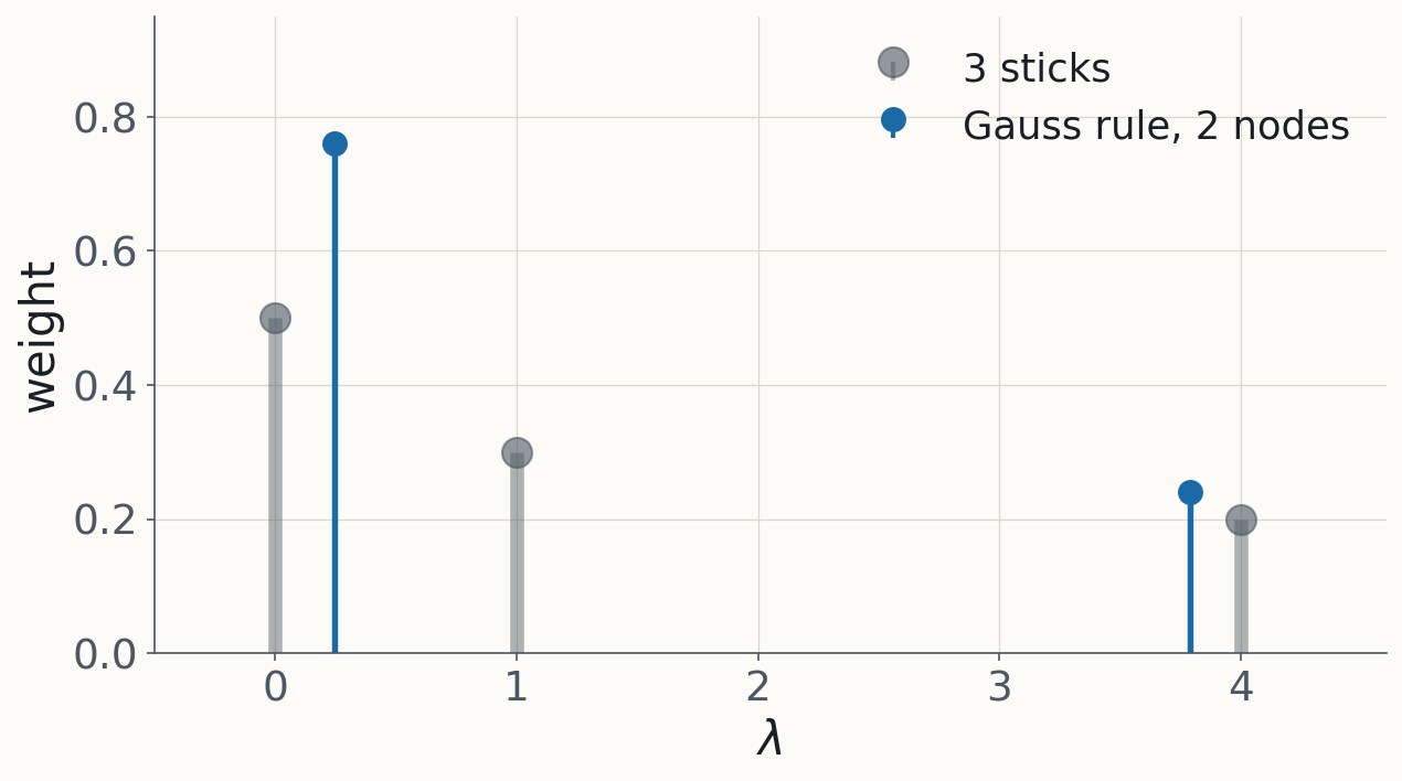
A three-atom measure and the two-node Gauss rule from Lanczos

Two nodes reproduce moments 0 to 3 of the three sticks exactly.

§3 · Stochastic Lanczos quadrature

Average the rules over a few random probes

$$\hat\rho(s)=\frac1{n_v}\sum_{\text{probes}}\ \sum_{k=1}^m\tau_k^2\,\delta(s-\theta_k)$$

Averaging $n_v$ random probes estimates $\rho$; finite $m$ adds quadrature error.

§3 · What SLQ sees

Ten steps place the outliers; the bulk needs more

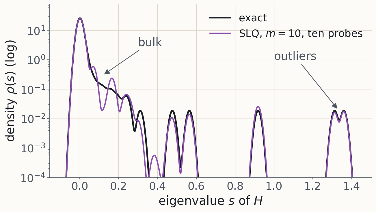
Exact spectral density against SLQ with m = 90, 30 and 10

Toy MLP: at $m=10$ the outliers are right and the bulk is lumpy.

§3 · Takeaway

A few probes times a few Lanczos steps give a spectral density: sharp outliers, blurry bulk.

§4 · Trained networks

What does the Hessian spectrum of a trained network look like?

§4 · Classifiers

A bulk and a few outliers

A bulk of eigenvalues near zero.
About $C$ large outliers, $C$ the number of classes.
The outliers come from class structure in $G$.

§4 · Language models

For a language model, $C$ is the vocabulary

$$C=|\text{vocabulary}|\approx10^4\text{–}10^5$$

"A few outliers" may be tens of thousands; $m=10$ cannot resolve them.

§4 · Takeaway

Classifiers: a bulk plus about $C$ outliers. Language models: still an open case.

§5 · Granziol & Juarev (2026)

How do you get $Hv$ from a 120B model sharded across GPUs?

§5 · The move

Finite differences, one shard at a time

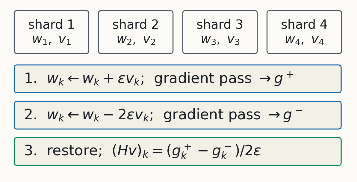
Four GPUs each holding a shard; perturb in place, two gradient passes, restore

Two ordinary gradient passes: a Lanczos step costs about two training steps.

§3.1, Algorithm 1. The only extra communication is scalar all-reduces for norms and dot products; $T_{Hv}\approx2T_{\rm grad}$. The gain is compatibility with the training stack, not FLOPs.

Cost (§5.1): Qwen-0.6B on one node, 1 → 8 GPUs gives 5.74× per HVP (Table 3); Lanczos bookkeeping adds 1.3–1.8% (Table 2); on 32B, Table 5 reports about 4× over HessFormer (89.6 s at batch 32 against 22.2 s at batch 80). HessFormer (Granziol 2025), the previous record: Pearlmutter HVPs on one 8-GPU node, SLQ on a 70B DeepSeek distilled model.

Reading the paper: "exact" means the true $H$, not a structured approximation; Figs 2–8 plot Ritz values against weights ("Gamma", "Ritz weights"), our $\theta_k$ and $\tau_k^2$; "smoothing parameter $\epsilon$" is the finite-difference step; their $\theta$ is the parameters and Pearlmutter's method is called "reverse-over-forward"; their loss is a dataset average; §4's Thm 4.1 assumes unbiased, independent finite-difference errors, while Thm 3.1 gives an $O(\epsilon^2)$ bias, so read §4 as heuristic.

§5 · Finding 1

The step size can fake a spectrum

$\epsilon=10^{-5}$ or $10^{-2}$: no separated outliers.
$\epsilon=10^{-4}$ or $10^{-3}$: clear outliers.
Which is right? Only an exact-$Hv$ check can say.

Pythia-160M, §7.1, Figs 3–6; the bad ones "resemble a random matrix". The authors attribute the failures to round-off and to averaging along the segment (Thm 3.1). But the "good" $\epsilon$ is the one that shows the expected outliers, and the check from slide 14 (finite difference against an exact HVP on a probe) is not reported, though it would be cheap at 160M.

Their Remark 3.2 puts fp32 $\epsilon^*$ at $10^{-3}$–$10^{-2}$, yet their sweet spot is $10^{-4}$–$10^{-3}$: constants and $\sqrt P$ move the optimum. fp32/bf16 labels in their figures refer to Lanczos-vector storage; bf16 storage is enough. 30× more data leaves the spectrum unchanged at fixed $\epsilon$ (Fig 7). They report Pythia-1.4B more stable in $\epsilon$ (Fig 8: $3\times10^{-4}$ to $10^{-2}$): one pair of models.

§5 · Finding 2

A 120B model shows large negative curvature

gpt-oss-120b: ten Lanczos steps, no $\epsilon$ sweep.
Real curvature, or an artefact of $\epsilon$ or Lanczos?
The authors call it "only indicative".

§5 · Finding 3

Per-layer (block-diagonal) curvature can be wrong by $O(1)$

$$\frac{\|(Hv)_b-H_{bb}v_b\|}{\|(Hv)_b\|}\ \approx\ 1$$

$b$: one transformer layer. Dropping cross-layer blocks loses about as much as it keeps.

§5 · Takeaway

At 120B the primitive still works; its knobs still need checking.

§6 · Back to attribution

What does the spectrum tell you about influence?

§6 · The IF in G's eigenbasis

In $G$'s eigenbasis $(s_k,u_k)$, each direction gets its own weight

$$\mathcal I_i=-\sum_k\frac{(u_k\cdot\nabla\phi)\,(u_k\cdot\nabla L_i)}{s_k+\lambda}$$

Far below $\lambda$: a scaled gradient dot product. Near or above: curvature-weighted.

§6 · Where λ sits

Where $\lambda$ sits decides which directions count as curvature

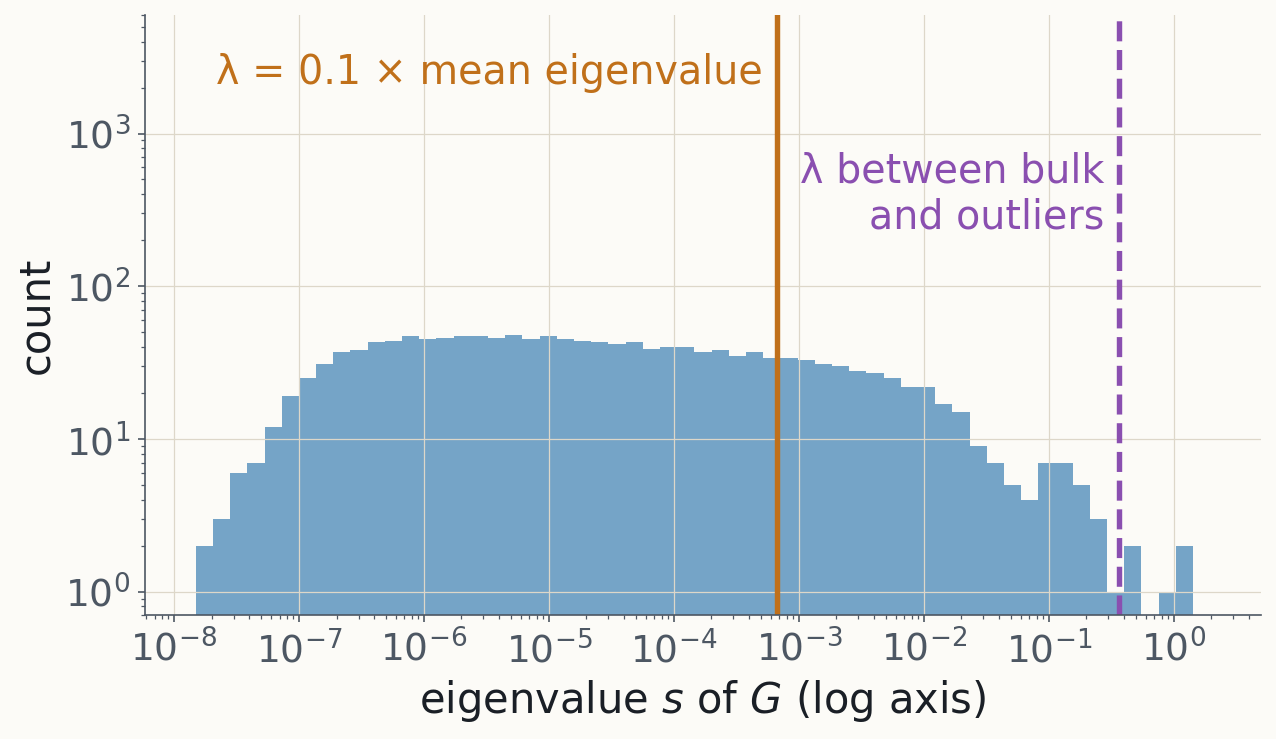
Eigenvalues of the toy's Gauss-Newton matrix with the damped filter at two dampings

Left of $\lambda$: a scaled gradient dot product. Right of it: curvature-weighted.

Toy $G$ (mean loss), log axis: the bulk spans about seven decades. Grosse et al. set $\lambda=0.1\times$ the mean EK-FAC eigenvalue, layer by layer; on the toy's exact $G$ that puts 78% of eigenvalues below $\lambda$. A $\lambda$ between bulk and outliers puts 99.7% below.

At scale both are computable: SLQ sees the outliers well, and the mean $\operatorname{tr}G/P$ comes from Hutchinson on $Gv$ (check its spread). Where $0.1\times$mean falls inside the bulk is what SLQ resolves least well. DA2's Code 1 sweeps $10^{-3}$ to $10^{-1}$ times the mean eigenvalue; DA1 §5's exercise uses the median Hessian eigenvalue.

$\lambda$ also has a meaning: DA1 §4's proximal penalty. Choosing it from the spectrum is a statement about where you trust the quadratic model; choosing it from the proximal target is a statement about the question.

(Room for the instructor's framing.)

§6 · Auditing

Check the approximation, not just the answer

EK-FAC assumes block-diagonal curvature.
Dropping cross-layer blocks already costs $O(1)$ in $Hv$.
Check against exact products: $Gv$ for EK-FAC, $Hv$ for Hessians.

§6 · Takeaway

The spectrum shows what your damping and your approximation are doing.

Summary

Three things to keep

$v\mapsto Hv$ costs a few gradients.
Lanczos and SLQ: outliers fast, a density from few probes.
Check step sizes and approximations against exact products.

Readings · Importance / Length

Granziol & Juarev 2026, Hessian Spectral Analysis at Foundation Model Scale ●●●●● / ●●●○○
Ghorbani, Krishnan & Xiao 2019, Hessian Eigenvalue Density ●●●●○ / ●●●○○
Pearlmutter 1994, Fast Exact Multiplication by the Hessian ●●●○○ / ●●○○○
Papyan 2020, Traces of Class/Cross-Class Structure ●●●○○ / ●●●●○
Wikipedia: Lanczos algorithm, Gaussian quadrature ●●●●○ / ●●○○○