SLT Notebook 1 — Bayesian inference as statistical mechanics
Singular Learning Theory, Iliad Intensive 2026
To run the code, open slt1_bayes_statmech.ipynb in Jupyter (CPU only; needs numpy, matplotlib and scipy). Every code cell's output is shown on this page; exercise solutions are folded under Solution.
These notebooks are a backup. The primary material is the original Iliad worksheet, Singular Learning Theory by Kai Ogden, Matthew Farrugia-Roberts and Zach Furman (with solutions, without), and Furman’s slides. Then the blog posts: Liam Carroll’s Distilling Singular Learning Theory (DSLT 0–4), Jesse Hoogland’s Neural networks generalize because of this one weird trick and, with Stan van Wingerden, You’re Measuring Model Complexity Wrong; and Zach Furman’s Singular learning theory: exercises. Come here for a derivation, a worked exercise, or code to check something.
Question: what does Bayes do with n samples, and how well does it generalize?
Route. 1.1 Bayes’ rule is a Boltzmann distribution. 1.2 The posterior becomes a Gaussian of width n^{-1/2}. 1.3 The free energy is the best fit plus \tfrac d2\log n. 1.4 Bayes generalizes with error d/2n; how maximum likelihood compares.
Setup. Data x_1,\dots,x_n are drawn i.i.d. from an unknown density q. A model p(x\mid w) has d parameters and a smooth positive prior \varphi(w).
| symbol | meaning |
|---|---|
| \ell(x,w)=-\log p(x\mid w) | per-sample loss |
| L_n(w)=\frac1n\sum_i\ell(x_i,w) | training loss |
| L(w)=\mathbb E_q\,\ell(x,w) | population loss, =S+\mathrm{KL}(q\,|\,p_w) |
| S=-\mathbb E_q\log q | entropy of the data |
| w_0, \hat w | minimizers of L and of L_n |
| K_n=L_n-L_n(w_0) | excess training loss |
The model is well specified if q=p_{w_0} and misspecified otherwise.
Code (13 lines)
import numpy as np
import matplotlib.pyplot as plt
from scipy.special import logsumexp

plt.rcParams.update({"figure.dpi": 110, "axes.grid": True, "grid.alpha": 0.3})
rng = np.random.default_rng(0)


def log_trapz(logf, x):
    # log of the trapezoid-rule integral of exp(logf) over the 1-D grid x,
    # computed in log space so that very small integrands do not underflow
    m = np.logaddexp(logf[:-1], logf[1:]) - np.log(2)
    return logsumexp(m + np.log(np.diff(x)))
1.1 The dictionary
Question: what does Bayes’ rule look like in the language of statistical mechanics?
Notation: prior \varphi, training loss L_n, population optimum w_0.
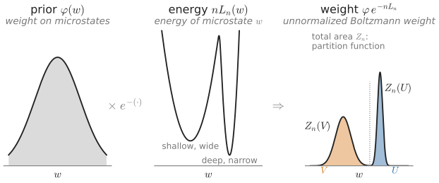
Prior times e^{-\text{energy}} gives an unnormalized weight whose total area is the partition function; the narrow well U is deeper but holds less mass than the wide well V.
The likelihood of the data is e^{-nL_n(w)}, so Bayes’ rule reads
\pi_n(w)=\frac{\varphi(w)\,e^{-nL_n(w)}}{Z_n}, \qquad Z_n=\int\varphi(w)\,e^{-nL_n(w)}\,dw, \qquad F_n=-\log Z_n .
This is a Boltzmann distribution. The total training loss nL_n is the energy and the prior weights the states. The evidence Z_n is the partition function, and the free energy is low when the model gave the data high probability.
Two variants are useful. A power \beta on the likelihood is an inverse temperature, with Bayes at \beta=1. Factoring out the loss at the population optimum, with K_n=L_n-L_n(w_0), leaves a free energy that measures how much prior mass fits the data nearly as well as w_0:
\pi_{n,\beta}\propto\varphi\,e^{-\beta nL_n}, \qquad F_n=nL_n(w_0)+\bar F_n, \qquad \bar F_n=-\log\int\varphi\,e^{-nK_n}\,dw .
| Bayesian statistics | statistical mechanics |
|---|---|
| parameter w | microstate |
| prior | a priori weight |
| nL_n(w) | energy |
| \beta | inverse temperature |
| posterior | Boltzmann distribution |
| evidence Z_n | partition function |
| F_n | free energy (units of k_BT) |
| posterior mean of nL_n | internal energy |
The analogy is formal: the energy is random because it depends on the sample, n is not a system size, and the real analogue of the density of states is the volume of parameters at a given loss (Notebook 2). The algebra, though, is exact.
Exercise 1.1 (Free-energy bookkeeping). For a region U of parameter space let F_n(U)=-\log\int_U\varphi e^{-nL_n}.
- Show that the log posterior odds of two regions are F_n(V)-F_n(U).
- If k regions partition parameter space and U_1 has the lowest free energy, show F_n(U_1)-\log k\le F_n\le F_n(U_1).
- Show that \partial_\beta F_n(\beta) is the internal energy n\,\mathbb E_\beta[L_n], and that F_n(\beta) is concave.
Solution
1. The posterior mass of U is e^{-F_n(U)}/Z_n. The Z_n cancels in the ratio.
2. Z_n=\sum_je^{-F_n(U_j)} lies between its largest term e^{-F_n(U_1)} and k times that term. Take -\log. Equal masses attain the lower bound.
3. Differentiate Z_n(\beta)=\int\varphi e^{-\beta nL_n}:
\partial_\beta F_n=-\frac{\partial_\beta Z_n}{Z_n}=\mathbb E_\beta[nL_n], \qquad \partial^2_\beta F_n=-\big(\mathbb E_\beta[(nL_n)^2]-\mathbb E_\beta[nL_n]^2\big)=-\mathrm{Var}_\beta[nL_n]\le0 .
1.2 Posterior concentration
Question: what does the posterior look like when n is large?
Notation: H=\nabla^2L(w_0) and H_n=\nabla^2L_n(\hat w) are Hessians; C=\mathrm{Cov}_q[\nabla\ell(x,w_0)] is the gradient covariance. The model is regular: w_0 is the unique minimizer and H is positive definite (plus the usual smoothness and moment conditions).
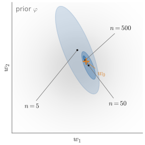
Schematic: the posterior’s Gaussian approximation for n=5,50,500 shrinks by \sqrt{10} per tenfold increase in n, and its centre settles near w_0.
As n grows the likelihood sharpens while the prior stays fixed. The posterior is squeezed onto \hat w, where only the quadratic part of the loss matters. The centre \hat w is itself random, since the training loss depends on the sample. Two Gaussian statements follow: the Bernstein–von Mises theorem, and the asymptotic normality of the maximum-likelihood estimate.
\pi_n\approx\mathcal N\big(\hat w,\,(nH_n)^{-1}\big), \qquad \hat w-w_0\approx\mathcal N\big(0,\,\tfrac1nH^{-1}CH^{-1}\big).
The first is what the posterior believes. The second is how the estimate actually varies between data sets. Both have width n^{-1/2}, and they agree when the model is well specified, because then C=H. Otherwise the posterior is over- or under-confident.
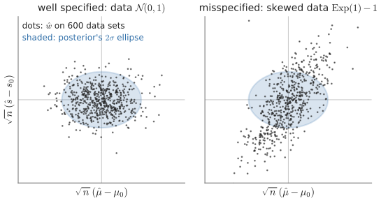
Model \mathcal N(\mu,e^{2s}), n=400, axes scaled by \sqrt n: the posterior’s ellipse (shaded, drawn at w_0) against the estimate on 600 data sets (dots), which agree when well specified and not for skewed data.
Exercise 1.2 (The Gaussian posterior).
- Expand nL_n to second order about \hat w, freeze the prior at its value there, and show that the posterior is the first Gaussian above. Writing w=\hat w+u/\sqrt n, show that the neglected terms are O(n^{-1/2}).
- Show that \hat w-w_0\approx-H^{-1}\nabla L_n(w_0), and use the central limit theorem to get the second Gaussian.
- Show that C=H when the model is well specified.
Hint
Differentiate \int p(x\mid w)\,dx=1 twice with respect to w.
Solution
1. With \delta=w-\hat w and a vanishing gradient at \hat w,
nL_n(w)=nL_n(\hat w)+\tfrac12\delta^\top(nH_n)\delta+O(n|\delta|^3).
Dropping the cubic term and freezing the prior leaves a Gaussian with covariance (nH_n)^{-1}. At \delta=u/\sqrt n the quadratic term is of order one, so the width is n^{-1/2}. On that scale the cubic term is n\cdot n^{-3/2}=n^{-1/2}, and a smooth prior also varies by O(n^{-1/2}).
2. Expand the first-order condition about w_0, with \nabla^2L_n(w_0)\to H:
0=\nabla L_n(\hat w)\approx\nabla L_n(w_0)+H(\hat w-w_0).
The gradient at w_0 is an average of n i.i.d. vectors with mean \nabla L(w_0)=0 and covariance C. By the central limit theorem it is approximately \mathcal N(0,C/n), and multiplying by -H^{-1} gives the covariance H^{-1}CH^{-1}/n.
3. One derivative gives \mathbb E_{p_w}[\nabla\log p]=0. A second, with \nabla^2p=p\,(\nabla^2\log p+\nabla\log p\,\nabla\log p^\top), gives
\mathbb E_{p_w}[\nabla^2\log p]+\mathbb E_{p_w}[\nabla\log p\,\nabla\log p^\top]=0 .
At w_0 with q=p_{w_0} the first term is -H and the second is C. Under misspecification H and C are expectations under q, not p_{w_0}, and the identity fails.
1.3 Laplace and the BIC
Question: what is the free energy for large n, and what does it penalize?
Notation: \hat w minimizes L_n, H_n is the Hessian there (positive definite: the model is regular, §1.2), d is the number of parameters.
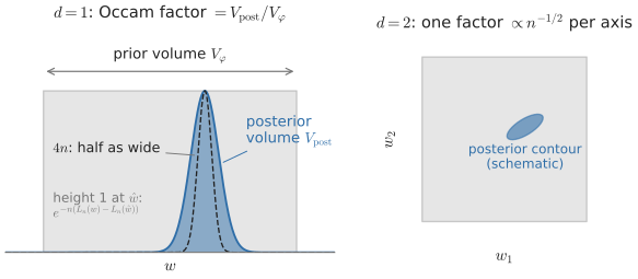
With a uniform prior the Occam factor is the posterior volume over the prior volume; quadrupling n halves each width, which is where \tfrac d2\log n comes from.
Laplace’s method replaces the integrand of Z_n by a Gaussian around \hat w (Exercise 1.3). The result is
F_n=nL_n(\hat w)+\frac d2\log n+\frac12\log\det H_n-\log\varphi(\hat w)-\frac d2\log2\pi+o(1).
The first two terms are the Bayesian information criterion (BIC): the best fit plus half a \log n per parameter. The rest is of order one; it depends on the curvature and the prior.
MacKay (1992) reads this as the best-fit likelihood times an Occam factor. For a uniform prior, the Occam factor is the fraction of prior volume that still fits the data. Each parameter’s width shrinks to about n^{-1/2}, and the evidence pays for the shrinkage. No held-out data are involved.
Exercise 1.3 (Laplace, BIC and the Occam factor).
- Using \int e^{-\frac12u^\top Au}\,du=(2\pi)^{d/2}(\det A)^{-1/2} for positive definite A, derive the formula for F_n.
- Take a uniform prior on a box of volume V_\varphi, and let V_{\rm post}=\int_{\rm box}e^{-n(L_n(w)-L_n(\hat w))}dw. Show that Z_n=e^{-nL_n(\hat w)}\,V_{\rm post}/V_\varphi exactly.
- Model B has more parameters than model A and fits better. Using the BIC, how much must B lower the per-sample training loss to be preferred? Compare with what fitting pure noise gains, about \tfrac1{2n} per extra parameter.
Solution
1. Expand to second order at \hat w and freeze the prior:
Z_n\approx\varphi(\hat w)\,e^{-nL_n(\hat w)}\int e^{-\frac12\delta^\top(nH_n)\delta}\,d\delta =\varphi(\hat w)\,e^{-nL_n(\hat w)}\Big(\frac{2\pi}n\Big)^{d/2}(\det H_n)^{-1/2},
using \det(nH_n)=n^d\det H_n. Take -\log. The error terms are those of Exercise 1.2.
2. On the box the prior is 1/V_\varphi; pull e^{-nL_n(\hat w)} out of the integral. Laplace then gives V_{\rm post}\approx(2\pi/n)^{d/2}(\det H_n)^{-1/2}, a width of order n^{-1/2} per parameter.
3. The BIC difference is
F^A-F^B\approx n\big(L_n^A-L_n^B\big)-\frac{d_B-d_A}2\log n .
So B wins only if it lowers the per-sample loss by more than \frac{\log n}{2n} per extra parameter. Fitting noise gains about \frac1{2n}, smaller by a factor \log n, so the BIC rejects parameters that only fit noise. A real improvement of fixed size wins once n is large.
Code. The first cell checks Laplace against the exact free energy of the conjugate model \mathcal N(w,1) with a Gaussian prior; the second computes F_n by quadrature for \mathcal N(\mu,e^{2s}) and checks the slope d/2=1 in \log n.
Code (18 lines)
# 1-D conjugate model: x ~ N(w, 1), prior w ~ N(0, tau^2). Exact Z_n vs quadrature vs Laplace.
tau2, n = 4.0, 50
x = rng.normal(1.0, 1.0, size=n)
xbar = x.mean()
nL_hat = 0.5 * n * np.log(2 * np.pi) + 0.5 * np.sum((x - xbar) ** 2)   # n L_n(w_hat)

F_exact = nL_hat + 0.5 * np.log(n) + 0.5 * np.log(tau2 + 1 / n) + xbar**2 / (2 * (tau2 + 1 / n))
F_laplace = nL_hat + 0.5 * np.log(n) + 0.5 * np.log(tau2) + xbar**2 / (2 * tau2)
F_bic = nL_hat + 0.5 * np.log(n)

w = np.linspace(-10, 10, 20001)
log_integrand = (-0.5 * w**2 / tau2 - 0.5 * np.log(2 * np.pi * tau2)
                 - 0.5 * n * np.log(2 * np.pi) - 0.5 * ((x[None, :] - w[:, None]) ** 2).sum(1))
F_quad = -log_trapz(log_integrand, w)
print(f"F_n exact     {F_exact:.4f}")
print(f"F_n quadrature{F_quad:.4f}")
print(f"F_n Laplace   {F_laplace:.4f}   (difference {F_laplace - F_exact:+.4f}, predicted O(1/n) ~ {1/(2*n*tau2):.4f})")
print(f"F_n BIC terms {F_bic:.4f}")
F_n exact 69.5111 F_n quadrature69.5111 F_n Laplace 69.5094 (difference -0.0017, predicted O(1/n) ~ 0.0025) F_n BIC terms 68.6570
Code (42 lines)
# 2-D model: x ~ N(mu, exp(2 s)), priors mu ~ N(0,1), s ~ N(0,1). Data from N(1, 0.5^2).
mu_true, sigma_true = 1.0, 0.5
N_all = 3000
x_all = rng.normal(mu_true, sigma_true, size=N_all)
mu_grid = np.linspace(-2.0, 4.0, 601)
s_grid = np.linspace(-4.0, 2.0, 601)
MU, S = np.meshgrid(mu_grid, s_grid, indexing="ij")
log_prior = -0.5 * (MU**2 + S**2) - np.log(2 * np.pi)
dmu, ds = mu_grid[1] - mu_grid[0], s_grid[1] - s_grid[0]

def free_energy_2d(x):
    n = len(x)
    # n L_n(mu, s) = n s + n/2 log 2pi + exp(-2s) * sum (x_i - mu)^2 / 2
    ss = ((x[None, None, :] - MU[:, :, None]) ** 2).sum(-1) if n <= 300 else \
         n * ((MU - x.mean()) ** 2 + x.var())           # same thing, computed from sufficient statistics
    nL = n * S + 0.5 * n * np.log(2 * np.pi) + 0.5 * np.exp(-2 * S) * ss
    return -(logsumexp(log_prior - nL) + np.log(dmu * ds))

def laplace_2d(x):
    n = len(x)
    mu_hat, s_hat = x.mean(), 0.5 * np.log(x.var())
    nL_hat = n * s_hat + 0.5 * n * np.log(2 * np.pi) + 0.5 * n       # exp(-2 s_hat) * n var = n
    H = np.diag([np.exp(-2 * s_hat), 2.0])                            # Hessian of L_n at the optimum
    F_lap = (nL_hat + 1.0 * np.log(n) + 0.5 * np.log(np.linalg.det(H))
             + 0.5 * (mu_hat**2 + s_hat**2) + np.log(2 * np.pi) - np.log(2 * np.pi))
    return nL_hat, F_lap

ns = np.array([10, 20, 50, 100, 200, 500, 1000, 2000, 3000])
rows = []
for n in ns:
    x = x_all[:n]
    nL_hat, F_lap = laplace_2d(x)
    rows.append((n, free_energy_2d(x) - nL_hat, F_lap - nL_hat, 1.0 * np.log(n)))
rows = np.array(rows)
plt.figure(figsize=(5.5, 3.6))
plt.plot(rows[:, 0], rows[:, 1], "o-", label="exact (quadrature)")
plt.plot(rows[:, 0], rows[:, 2], "s--", label="Laplace")
plt.plot(rows[:, 0], rows[:, 3], ":", label=r"BIC: $\frac{d}{2}\log n$")
plt.xscale("log"); plt.xlabel("n"); plt.ylabel(r"$F_n - nL_n(\hat w)$")
plt.title("2-parameter Gaussian model: free energy above the best fit"); plt.legend(); plt.tight_layout(); plt.show()
print("slope of the exact curve against log n over the last four points:",
      np.polyfit(np.log(rows[-4:, 0]), rows[-4:, 1], 1)[0].round(3), " (d/2 = 1)")
slope of the exact curve against log n over the last four points: 1.009 (d/2 = 1)
1.4 The Bayes generalization error
Question: how well does the posterior predict the next sample, compared with the maximum-likelihood fit?
Notation: L is the population loss, minimized at w_0; \hat w minimizes the training loss; S is the entropy of the data; \pi_n is the posterior and F_n the free energy (§1.1); H and C are the Hessian and gradient covariance at w_0; L_{\min}=L(w_0)-S is the best excess loss the model can reach (zero if well specified).
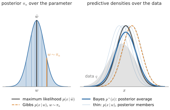
Maximum likelihood predicts with the fitted member, Gibbs with one random member, and Bayes with the posterior average, which here is wider than either (Exercise 1.4.3 at n=4).
There are three predictors. Bayes averages the model over the posterior, giving the predictive density p^*. Gibbs uses one posterior sample. Maximum likelihood uses \hat w. Each one’s generalization error G_n is its expected loss on a fresh sample minus the entropy, which no predictor can remove. The results below also average over training sets.
The free energy enters through an exact identity (Exercise 1.4.1):
p^*(x)=\int p(x\mid w)\,\pi_n(w)\,dw, \qquad -\log p^*(x_{n+1})=F_{n+1}-F_n .
In the regular case, up to o(1/n):
| predictor | expected generalization error |
|---|---|
| Bayes | L_{\min}+\dfrac{d}{2n} |
| Gibbs | L_{\min}+\dfrac{d+\mathrm{tr}(H^{-1}C)}{2n} |
| maximum likelihood | L_{\min}+\dfrac{\mathrm{tr}(H^{-1}C)}{2n} |
When the model is well specified the trace is d. Bayes and maximum likelihood then tie, and one posterior sample pays twice as much. Under misspecification Bayes still pays d/2n, while maximum likelihood can pay more or less. So Bayes does not always generalize better; what posterior averaging removes is the dependence on C.
Exercise 1.4 (Three generalization errors).
- Prove -\log p^*(x_{n+1})=F_{n+1}-F_n.
- Derive the table. Start from the fluctuation of \hat w (§1.2) for the maximum-likelihood row, then add the posterior spread for Gibbs. For Bayes, expand \log p(x\mid w) to second order about \hat w and use \log\mathbb E[e^Y]\approx\mathbb E[Y]+\tfrac12\mathrm{Var}[Y].
- (Misspecified.) Model \mathcal N(x;w,1), flat prior, data \mathcal N(0,\sigma^2). Compute the three expected errors exactly. When does Bayes beat maximum likelihood?
Solution
1. Adding a point multiplies the integrand by p(x_{n+1}\mid w), so Z_{n+1}=Z_n\int p(x_{n+1}\mid w)\,\pi_n(w)\,dw=Z_n\,p^*(x_{n+1}). Take -\log.
2. Maximum likelihood. Expand L about w_0 and use the covariance of \hat w:
\mathbb E[L(\hat w)]-L(w_0)\approx\tfrac12\,\mathbb E\big[(\hat w-w_0)^\top H(\hat w-w_0)\big]=\frac{\mathrm{tr}(H^{-1}C)}{2n}.
Gibbs. A posterior sample sits a further \delta\sim\mathcal N(0,(nH)^{-1}) from \hat w, which adds \tfrac12\mathbb E[\delta^\top H\delta]=\frac d{2n}.
Bayes. Write \log p(x\mid\hat w+\delta)\approx-\ell(x,\hat w)+s^\top\delta+\tfrac12\delta^\top M\delta, with s and M the gradient and Hessian of \log p at \hat w. Average over the posterior, then over x\sim q; inside the 1/n terms replace \hat w by w_0, where \mathbb E_q[ss^\top]=C and \mathbb E_q[M]=-H:
-\log p^*(x)\approx\ell(x,\hat w)-\frac{s^\top H^{-1}s+\mathrm{tr}(H^{-1}M)}{2n}, \qquad \mathbb E_x[-\log p^*(x)]\approx L(\hat w)-\frac{\mathrm{tr}(H^{-1}C)-d}{2n}.
Averaging over training sets adds the maximum-likelihood term. The two trace terms cancel, leaving L(w_0)+\frac d{2n}.
3. The posterior is \mathcal N(\bar x,1/n) and the predictive is \mathcal N(\bar x,1+1/n). Here H=1, C=\sigma^2, and
L(w)-S=\tfrac12\big(w^2+\sigma^2-1-\log\sigma^2\big), \qquad L_{\min}=\tfrac12\big(\sigma^2-1-\log\sigma^2\big).
With \mathbb E[\bar x^2]=\sigma^2/n, the expected errors above L_{\min} are
\text{MLE: }\frac{\sigma^2}{2n}, \qquad \text{Gibbs: }\frac{\sigma^2+1}{2n}, \qquad \text{Bayes: }\tfrac12\log\big(1+\tfrac1n\big)=\frac1{2n}+O(n^{-2}).
Bayes beats maximum likelihood when \sigma^2>n\log(1+1/n), a threshold just below 1. Averaging helps when the data are noisier than the model assumes.
Code. Simulates Exercise 1.4.3 and plots n times each expected error; the dotted lines are the table. Set sigma2 below 1 to see Bayes and maximum likelihood swap.
sigma2 = 2.0          # variance of the data; the model assumes 1
tau2 = 100.0          # prior variance (wide, so the prior barely matters)
ns = np.array([5, 10, 20, 50, 100, 200, 500])
trials = 4000
S = 0.5 * np.log(2 * np.pi * np.e * sigma2)
L_min = 0.5 * (sigma2 - 1 - np.log(sigma2))

def errors(xbar, n):
    # TODO: return (G_bayes, G_gibbs, G_mle) minus L_min, given the sample mean xbar
    # posterior: N(m, v) with v = 1 / (n + 1/tau2), m = v * n * xbar; predictive: N(m, 1 + v)
    raise NotImplementedError

# then: average over trials for each n and plot n * G against n, with the three predicted lines
Solution (code)
sigma2 = 2.0          # variance of the data; the model assumes 1
tau2 = 100.0          # prior variance (wide, so the prior barely matters)
ns = np.array([5, 10, 20, 50, 100, 200, 500])
trials = 4000
S = 0.5 * np.log(2 * np.pi * np.e * sigma2)
L_min = 0.5 * (sigma2 - 1 - np.log(sigma2))

def errors(xbar, n):
    v = 1.0 / (n + 1.0 / tau2)
    m = v * n * xbar
    # expected loss of a Gaussian predictor N(m, s2) on x ~ N(0, sigma2): 1/2 log(2 pi s2) + (sigma2 + m^2) / (2 s2)
    bayes = 0.5 * np.log(2 * np.pi * (1 + v)) + (sigma2 + m**2) / (2 * (1 + v)) - S - L_min
    gibbs = 0.5 * np.log(2 * np.pi) + 0.5 * (sigma2 + m**2 + v) - S - L_min
    mle = 0.5 * np.log(2 * np.pi) + 0.5 * (sigma2 + xbar**2) - S - L_min
    return bayes, gibbs, mle

means = []
for n in ns:
    xbar = rng.normal(0.0, np.sqrt(sigma2 / n), size=trials)
    means.append([np.mean(g) for g in errors(xbar, n)])
means = np.array(means)

plt.figure(figsize=(5.5, 3.6))
for j, (lab, pred) in enumerate([("Bayes predictive", 0.5), ("Gibbs (one sample)", (1 + sigma2) / 2),
                                 ("maximum likelihood", sigma2 / 2)]):
    plt.plot(ns, ns * means[:, j], "o-", color=f"C{j}", label=lab)
    plt.axhline(pred, color=f"C{j}", ls=":")
plt.xscale("log"); plt.xlabel("n"); plt.ylabel(r"$n\,\mathbb{E}[G_n - L_{\min}]$")
plt.title(f"model N(w,1), data N(0,{sigma2}); dotted = table"); plt.legend(loc="center right"); plt.tight_layout(); plt.show()