SLT Notebook 2 — Free energy and basin volume
Singular Learning Theory, Iliad Intensive 2026
To run the code, open slt2_free_energy_volume.ipynb in Jupyter (CPU only; needs numpy, matplotlib and scipy). Every code cell's output is shown on this page; exercise solutions are folded under Solution.
These notebooks are a backup. The primary material is the original Iliad worksheet, Singular Learning Theory by Kai Ogden, Matthew Farrugia-Roberts and Zach Furman (with solutions, without), and Furman’s slides. Then the blog posts: Liam Carroll’s Distilling Singular Learning Theory (DSLT 0–4), Jesse Hoogland’s Neural networks generalize because of this one weird trick and, with Stan van Wingerden, You’re Measuring Model Complexity Wrong; and Zach Furman’s Singular learning theory: exercises. Come here for a derivation, a worked exercise, or code to check something.
Question: when the Hessian at the minimum is degenerate, what replaces \tfrac d2\log n in the free energy?
Route: 2.1 the answer is a volume exponent; 2.2 how to compute it from a transform; 2.3 what it does when there are several basins.
Notation (as in Notebook 1). Parameter w\in\mathbb R^d, prior \varphi, excess population loss K=L-L(w_0)\ge0.
\bar Z_n=\int\varphi(w)\,e^{-nK(w)}\,dw,\qquad \bar F_n=-\log\bar Z_n .
We use the population loss in place of the training loss throughout. Under Watanabe’s assumptions this changes the free energy only by a random O(1), so the coefficients of \log n are unaffected.
Code (14 lines)
import numpy as np
import matplotlib.pyplot as plt
from scipy.special import logsumexp, gammaln

plt.rcParams.update({"figure.dpi": 110, "axes.grid": True, "grid.alpha": 0.3})


def log_Zbar(logphi_grid, K_grid, cell, n):
    # log of  sum_grid  phi * exp(-n K) * cell volume,  a Riemann sum for Zbar_n; log space avoids underflow
    return logsumexp(logphi_grid - n * K_grid) + np.log(cell)


def slope(xs, ys):
    return np.polyfit(xs, ys, 1)[0]
2.1 Volume scaling
Question: what property of the loss sets the coefficient of \log n?
Notation: \bar Z_n, \bar F_n as above. New: the prior volume of a sublevel set, and its derivative,
V(t)=\int_{K(w)<t}\varphi(w)\,dw,\qquad v(t)=V'(t).
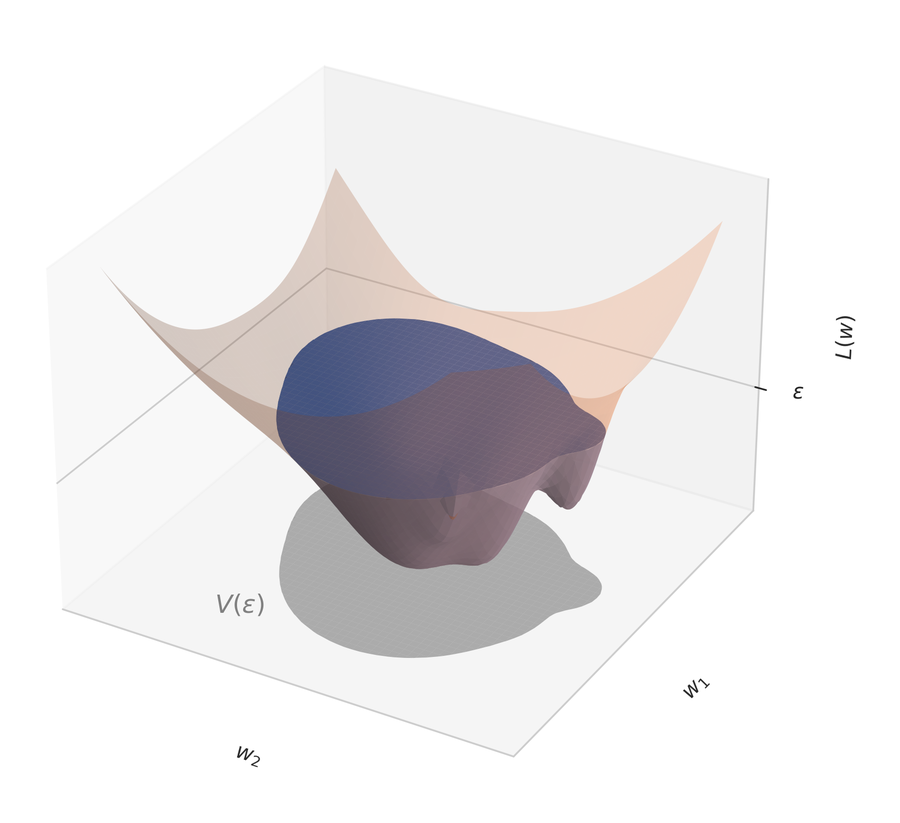
The part of a loss surface below a threshold, projected onto parameter space (grey), has volume V(\epsilon). Figure from Jesse Hoogland and Stan van Wingerden, You’re Measuring Model Complexity Wrong (LessWrong, 2023).
Slice by loss. The integrand of the partition function depends on a parameter only through its loss. Grouping parameters by loss level turns a d-dimensional integral into a one-dimensional one:
\bar Z_n=\int_0^\infty e^{-nt}\,v(t)\,dt=n\int_0^\infty e^{-nt}\,V(t)\,dt .
In the dictionary of Notebook 1, v is the density of states. The weight e^{-nt} kills every level above about 1/n, so at large n only the volume of nearly optimal parameters matters.
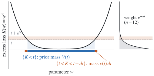
The sublevel set (blue) has volume V(t), the slab above it (orange) has volume v(t)\,dt, and \bar Z_n weights each slab by e^{-nt}.
The learning coefficient. Suppose the volume shrinks like a power, possibly with a logarithm. Then the free energy follows (Exercise 2.1.1):
V(t)\approx c\,t^{\lambda}(-\log t)^{m-1}\ (t\to0) \quad\Longrightarrow\quad \bar F_n=\lambda\log n-(m-1)\log\log n+O(1).
The exponent \lambda is the learning coefficient and m its multiplicity. For analytic losses and priors, Watanabe proved that the volume always has this form, with \lambda rational.
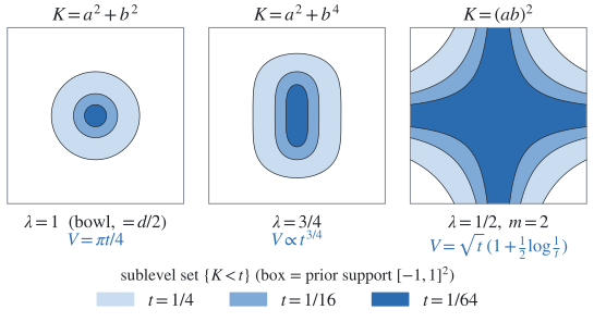
Sublevel sets at t=1/4,1/16,1/64: the flatter the valley, the slower the volume shrinks and the smaller \lambda.
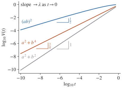
\lambda is the slope of \log V against \log t as t\to0; the logarithm in the cross’s volume makes it approach \tfrac12 slowly.
Bowl versus valley. A quadratic bowl has ellipsoidal sublevel sets of volume \propto t^{d/2}, so \lambda=d/2 and Notebook 1’s formula returns. Flat directions make the sublevel sets fatter and the exponent smaller. If the prior is positive at the minimum, \lambda\le d/2, with equality in the regular case. The Hessian cannot see any of this: it is zero for w^4 and w^6 alike.
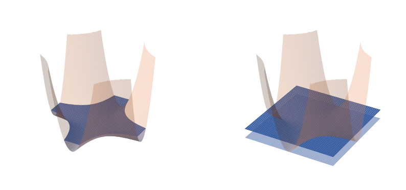
The real sublevel set of a degenerate basin (left), and the infinite slab the quadratic approximation predicts (right). Figure from Jesse Hoogland and Stan van Wingerden, You’re Measuring Model Complexity Wrong (LessWrong, 2023).
Exercise 2.1 (Volume and free energy). Use the uniform prior on [-1,1]^d.
- Derive the slicing formula. Then show that V=ct^\lambda near t=0 gives \bar F_n=\lambda\log n-\log(c\,\Gamma(\lambda+1))+o(1), with \Gamma the Gamma function.
Hint
Write e^{-nK}=n\int_K^\infty e^{-nt}dt and swap the integrals; then substitute t=s/n. - Compute V(t), \lambda and m for K=w^2, K=w^4 and K=(ab)^2.
- (Upper bound.) Let w_0 be an interior minimum where the prior is continuous and positive, and \Lambda a bound on the Hessian’s eigenvalues near w_0. Show that for small t the sublevel set contains a ball of radius \sqrt{2t/\Lambda}, and conclude \lambda\le d/2.
Solution
1. Swapping the order of integration,
\bar Z_n=\int\varphi(w)\,n\!\int_{K(w)}^\infty e^{-nt}dt\,dw=n\int_0^\infty e^{-nt}V(t)\,dt .
Integrating by parts gives the form with v. With V=ct^\lambda and t=s/n, the integral is c\,\Gamma(\lambda+1)\,n^{-\lambda}; take -\log. A factor (-\log t)^{m-1} becomes (\log n)^{m-1} to leading order, which gives the \log\log n term.
2. The prior density is 2^{-d}.
- w^2: the set is |w|<\sqrt t, so V=\sqrt t, \lambda=\tfrac12, m=1.
- w^4: V=t^{1/4}, \lambda=\tfrac14, m=1.
- (ab)^2: the set is |ab|<\sqrt t. For |a|<\sqrt t any b works; otherwise |b|<\sqrt t/|a|. Adding up,
V(t)=\tfrac12\sqrt t\,\log(1/t)+\sqrt t ,
so \lambda=\tfrac12 and m=2. The logarithm comes from the crossing of the two zero lines.
3. Taylor’s theorem with the remainder gives K(w)\le\tfrac12\Lambda\|w-w_0\|^2, so the ball of radius \sqrt{2t/\Lambda} lies in the sublevel set. Its prior volume is at least a constant times t^{d/2}. Since \log t<0, a larger volume means a smaller ratio \log V/\log t, so \lambda\le d/2.
Code. This cell checks the slope of \bar F_n against \log n for four toy losses (w^2+v^4 has \lambda=\tfrac12+\tfrac14); the \log\log n term biases the plain slope for (ab)^2.
Code (22 lines)
w1 = np.linspace(-1, 1, 400_001)                      # 1-D grid
A, B = np.meshgrid(np.linspace(-1, 1, 2001), np.linspace(-1, 1, 2001), indexing="ij")   # 2-D grid
ns = np.logspace(1, 4, 13)

toys = {
    r"$w^2$ ($\lambda=1/2$)":        (np.full_like(w1, np.log(0.5)), w1**2, w1[1] - w1[0], 0.5, 1),
    r"$w^4$ ($\lambda=1/4$)":        (np.full_like(w1, np.log(0.5)), w1**4, w1[1] - w1[0], 0.25, 1),
    r"$w^2+v^4$ ($\lambda=3/4$)":    (np.full_like(A, np.log(0.25)), A**2 + B**4, (A[1, 0] - A[0, 0]) ** 2, 0.75, 1),
    r"$(ab)^2$ ($\lambda=1/2,\,m=2$)": (np.full_like(A, np.log(0.25)), (A * B) ** 2, (A[1, 0] - A[0, 0]) ** 2, 0.5, 2),
}
plt.figure(figsize=(6, 3.8))
for label, (logphi, K, cell, lam, m) in toys.items():
    Fbar = np.array([-log_Zbar(logphi, K, cell, n) for n in ns])
    plt.plot(np.log(ns), Fbar, "o-", ms=4, label=label)
    big = ns >= 300
    s_plain = slope(np.log(ns[big]), Fbar[big])
    # fit  Fbar = lam * log n - (m-1) log log n + c  with the known m, to recover lam
    X = np.stack([np.log(ns[big]), np.ones(big.sum())], 1)
    s_full = np.linalg.lstsq(X, Fbar[big] + (m - 1) * np.log(np.log(ns[big])), rcond=None)[0][0]
    print(f"{label:34s} slope vs log n (n>=300): {s_plain:.3f};  with the log log n term: {s_full:.3f};  lambda = {lam}")
plt.xlabel(r"$\log n$"); plt.ylabel(r"$\bar F_n$"); plt.legend(); plt.title("free energy of four toy losses, uniform prior")
plt.tight_layout(); plt.show()
$w^2$ ($\lambda=1/2$) slope vs log n (n>=300): 0.500; with the log log n term: 0.500; lambda = 0.5 $w^4$ ($\lambda=1/4$) slope vs log n (n>=300): 0.250; with the log log n term: 0.250; lambda = 0.25 $w^2+v^4$ ($\lambda=3/4$) slope vs log n (n>=300): 0.750; with the log log n term: 0.750; lambda = 0.75 $(ab)^2$ ($\lambda=1/2,\,m=2$) slope vs log n (n>=300): 0.393; with the log log n term: 0.529; lambda = 0.5

2.2 The Mellin transform
Question: can we read off \lambda and m without computing the volume?
Notation: K, \varphi, v as in §2.1. New: the zeta function, for complex z,
\zeta(z)=\int K(w)^z\,\varphi(w)\,dw=\int_0^\infty t^z\,v(t)\,dt .
The second form is the slicing of §2.1 again. It says \zeta is the Mellin transform of the density of states, the analogue of a Fourier transform for powers of t.
Poles are terms. The integral converges for \mathrm{Re}\,z>0. Moving left, it first blows up where t^zv(t) stops being integrable at t=0. One integral makes this precise (Exercise 2.2.1):
\int_0^1 t^{z}\,t^{\lambda-1}(-\log t)^{m-1}\,dt=\frac{(m-1)!}{(z+\lambda)^m}.
So a term t^{\lambda-1}(-\log t)^{m-1} in the density of states is a pole of order m at -\lambda. By §2.1 the same term gives n^{-\lambda}(\log n)^{m-1} in the partition function.
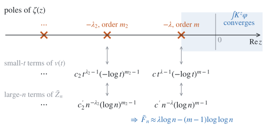
Each pole of \zeta matches a term of v near t=0 and a term of \bar Z_n at large n; the first pole gives \lambda and m.
The pole nearest the origin gives \lambda, its order gives m, and the poles further left give corrections. Watanabe proved that for analytic losses and priors these poles are all at negative rational numbers.
Monomials take one line. For a monomial the integral factorizes. For K=(ab)^2 with the uniform prior on [-1,1]^2,
\zeta(z)=\frac14\Big(\int_{-1}^1 a^{2z}da\Big)^2=\frac1{(2z+1)^2},
a double pole at -\tfrac12. So \lambda=\tfrac12 and m=2, without the case analysis of Exercise 2.1.2.
Exercise 2.2 (Poles). Uniform prior on [-1,1]^d unless stated.
- Prove the displayed integral.
Hint
Substitute t=e^{-u}. - Find the poles of \zeta for K=w_1^{2k_1}w_2^{2k_2}, and state the rule for \lambda and m.
- (Reparametrization.) The model K=\tfrac12\theta^2 is regular. Write \theta=\mu^3, so K=\tfrac12\mu^6, with a uniform prior on \mu. Find \lambda. Is \lambda a property of the set of distributions?
- With a standard normal prior and K=w^2, find all the poles of \zeta. What do the poles after the first one give?
Hint
\mathbb E|w|^{p}=2^{p/2}\Gamma(\tfrac{p+1}2)/\sqrt\pi, and \Gamma has poles at 0,-1,-2,\dots
Solution
1. With t=e^{-u} the integral becomes \int_0^\infty e^{-(z+\lambda)u}u^{m-1}du=(m-1)!/(z+\lambda)^m.
2. The integral factorizes:
\zeta(z)=\frac1{(2k_1z+1)(2k_2z+1)} .
The poles are at -1/2k_1 and -1/2k_2. So \lambda=\min_i 1/2k_i, and m is the number of i attaining the minimum. The same rule holds in d variables. A parameter that does not appear contributes nothing: flat directions are free.
3. \zeta(z)=2^{-z}/(6z+1), a pole at -\tfrac16, so \lambda=\tfrac16 rather than \tfrac12. Both coordinates describe the same distributions. A uniform prior on \mu, though, is a different prior from a uniform one on \theta. So \lambda belongs to the model together with its prior, not to the set of distributions alone.
4. \zeta(z)=\mathbb E[w^{2z}]=2^z\Gamma(z+\tfrac12)/\sqrt\pi, with simple poles at -\tfrac12,-\tfrac32,-\tfrac52,\dots. The first gives \lambda=\tfrac12. The others give the 1/n, 1/n^2,\dots corrections. Indeed here \bar Z_n=(1+2n)^{-1/2} exactly.
2.3 Several basins
Question: when the loss has several basins of different depth and width, where does the posterior go as n grows?
Notation: basins U_\alpha, each with minimum loss L_\alpha, learning coefficient \lambda_\alpha, and local free energy F_n(U_\alpha)=-\log\int_{U_\alpha}\varphi e^{-nL} (Notebook 1, Exercise 1.1), with constant term c_\alpha; \pi_n\propto\varphi e^{-nL} the posterior and \pi_n(U) its mass in U.
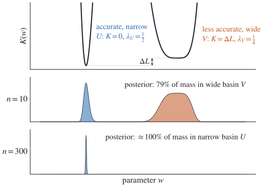
At small n the wide basin holds most of the posterior; at large n the accurate one takes over.
Accuracy against volume. Applying §2.1 inside each basin (multiplicity one for simplicity),
F_n(U_\alpha)\approx nL_\alpha+\lambda_\alpha\log n+c_\alpha,\qquad F_n\approx\min_\alpha F_n(U_\alpha).
Posterior mass is exponential in minus the free energy, so the posterior sits in the basin of least free energy. That basin balances accuracy (the term linear in n) against volume (the logarithm).
The switch. Take a narrow, accurate basin U and a wide, less accurate basin V. Write \Delta L=L_V-L_U>0 and \Delta\lambda=\lambda_U-\lambda_V>0. Keeping the leading terms (multiplicity one, constants dropped),
\log\frac{\pi_n(U)}{\pi_n(V)}\approx n\,\Delta L-\Delta\lambda\log n, \qquad \frac{n^*}{\log n^*}=\frac{\Delta\lambda}{\Delta L}.
If \Delta\lambda/\Delta L>e, the logarithm wins at first and the posterior sits in the wide basin. Past n^* the linear term wins and it moves to the accurate one. With real data each basin’s summed training loss fluctuates by O(\sqrt n), which blurs the switch.
In thermodynamic language. The derivative of the free energy in n is the mean excess loss under the posterior (Exercise 2.3.2). Near n^* that mean drops from about \Delta L to nearly zero. The dictionary calls such a kink in the free energy a first-order transition. The analogy stops there: no thermodynamic limit makes the kink sharp. The posterior also has no dynamics, so it is never stuck. Only a sampler or optimizer that moves locally can stay in the wide basin past n^*, which is metastability.
Exercise 2.3 (Two basins).
- Suppose F_n(U)\approx0.3n+20\log n and F_n(V)\approx0.5n+2\log n. Which basin is accurate and which is wide? Find n^*, and the posterior odds at n=100 and n=2000.
- Show that \partial_n\bar F_n is the posterior mean of K, and that in one basin it is about \lambda/n.
- (A staircase.) Three basins have (L_\alpha,\lambda_\alpha)=(0,2), (0.01,1) and (0.05,\tfrac14). Which holds the posterior as n runs from 10 to 10^5?
Solution
1. U is accurate (0.3<0.5) and narrow (20>2). With \Delta L=0.2 and \Delta\lambda=18, solve n/\log n=90: n^*\approx570. The log-odds for U are 0.2n-18\log n:
- at n=100, -63: the posterior is in V;
- at n=2000, +263: it is in U.
The log-odds cross from -5 to +5 within about 60 samples of n^*.
2. Differentiate under the integral:
\partial_n\bar F_n=\frac{\int K\varphi e^{-nK}}{\int\varphi e^{-nK}}=\mathbb E_{\pi_n}[K].
In one basin, \bar F_n\approx\lambda\log n gives \mathbb E_{\pi_n}[K]\approx\lambda/n. This is the equipartition of the problem, with \lambda in place of d/2; Notebook 3’s estimator is built on it.
3. Solve n/\log n=\Delta\lambda/\Delta L for each pair. Basins 3 and 2 cross at n\approx83, basins 2 and 1 at n\approx650. So the posterior is in basin 3 up to about 83, in basin 2 up to about 650, and in basin 1 after that. Each step is more accurate and narrower.
Code. The first cell follows the posterior across the switch for the loss in the figure (with \delta=0.01); the second plots Exercise 2.3.1.
Code (27 lines)
delta = 0.01
w = np.linspace(-2.5, 2.5, 200_001)
x = np.clip(w + 0.5, 0, 1)
step = x**3 * (10 - 15 * x + 6 * x**2)              # smooth step: 0 for w <= -1/2, 1 for w >= 1/2
K = (w + 1) ** 2 * (w - 1) ** 4 + delta * step
logphi = np.full_like(w, -np.log(5.0))            # uniform prior on [-2.5, 2.5]
dw = w[1] - w[0]
ns = np.logspace(0.5, 3.5, 61)
right_mass, Fbar, EK = [], [], []
for n in ns:
    logp = logphi - n * K
    logZ = logsumexp(logp) + np.log(dw)
    p = np.exp(logp - logZ) * dw
    right_mass.append(p[w > 0].sum()); Fbar.append(-logZ); EK.append((p * K).sum())
# n* from  n / log n = (1/2 - 1/4) / delta
target = 0.25 / delta
n_star = ns[np.argmin(np.abs(ns / np.log(ns) - target))]

fig, ax = plt.subplots(1, 3, figsize=(11, 3.3))
ax[0].plot(ns, right_mass); ax[0].axvline(n_star, color="k", ls=":", label=f"$n^*\\approx{n_star:.0f}$")
ax[0].set_xscale("log"); ax[0].set_xlabel("n"); ax[0].set_ylabel("posterior mass of the wide basin (w > 0)"); ax[0].legend()
ax[1].plot(np.log(ns), Fbar); ax[1].set_xlabel(r"$\log n$"); ax[1].set_ylabel(r"$\bar F_n$")
ax[2].loglog(ns, EK, label=r"$\mathbb{E}_{\pi_n}[K]$")
ax[2].loglog(ns, delta + 0.25 / ns, ":", label=r"wide basin: $\delta + \lambda_V/n$, $\lambda_V=1/4$")
ax[2].loglog(ns, 0.5 / ns, ":", label=r"narrow basin: $\lambda_U/n$, $\lambda_U=1/2$")
ax[2].set_xlabel("n"); ax[2].legend(fontsize=8); ax[2].axvline(n_star, color="k", ls=":")
plt.tight_layout(); plt.show()
# Exercise 2.3.1: plot F_n(U), F_n(V), the exact F_n = -log(e^{-F_U} + e^{-F_V}), and dF_n/dn, for n in [10, 3000].
n = np.linspace(10, 3000, 3000)
F_U = 0.3 * n + 20 * np.log(n)
F_V = 0.5 * n + 2 * np.log(n)
# TODO: F_total, the minimum of the two, and the derivative dF_total/dn (np.gradient); mark n* ~ 570
Solution (code)
n = np.linspace(10, 3000, 3000)
F_U = 0.3 * n + 20 * np.log(n)
F_V = 0.5 * n + 2 * np.log(n)
F_tot = -np.logaddexp(-F_U, -F_V)
fig, ax = plt.subplots(1, 2, figsize=(9, 3.3))
ax[0].plot(n, F_tot - 0.3 * n, label=r"$F_n - 0.3n$ (exact)")
ax[0].plot(n, np.minimum(F_U, F_V) - 0.3 * n, "--", label=r"$\min(F_U, F_V) - 0.3n$")
ax[0].axvline(570, color="k", ls=":"); ax[0].set_xlabel("n"); ax[0].legend()
ax[1].plot(n, np.gradient(F_tot, n)); ax[1].axhline(0.5, ls=":", color="C1"); ax[1].axhline(0.3, ls=":", color="C1")
ax[1].axvline(570, color="k", ls=":"); ax[1].set_xlabel("n"); ax[1].set_ylabel(r"$dF_n/dn$")
plt.tight_layout(); plt.show()
print("log posterior odds U:V at n = 100, 570, 2000:", [round(float(0.2 * m - 18 * np.log(m)), 1) for m in (100, 570, 2000)])
log posterior odds U:V at n = 100, 570, 2000: [-62.9, -0.2, 263.2]