SLT Notebook 3 — Effective exponents and temperature
Singular Learning Theory, Iliad Intensive 2026
To run the code, open slt3_effective_temperature.ipynb in Jupyter (CPU only; needs numpy, matplotlib and scipy). Every code cell's output is shown on this page; exercise solutions are folded under Solution.
These notebooks are a backup. The primary material is the original Iliad worksheet, Singular Learning Theory by Kai Ogden, Matthew Farrugia-Roberts and Zach Furman (with solutions, without), and Furman’s slides. Then the blog posts: Liam Carroll’s Distilling Singular Learning Theory (DSLT 0–4), Jesse Hoogland’s Neural networks generalize because of this one weird trick and, with Stan van Wingerden, You’re Measuring Model Complexity Wrong; and Zach Furman’s Singular learning theory: exercises. Come here for a derivation, a worked exercise, or code to check something.
Question: the learning coefficient \lambda is defined as n\to\infty. What does a finite sample measure?
Route. 3.1: a loss whose \lambda jumps, and the effective exponent a finite sample sees. 3.2: estimating it by sampling a tempered, localized posterior.
Code (27 lines)
import numpy as np
import matplotlib.pyplot as plt
from scipy.special import logsumexp

plt.rcParams.update({"figure.dpi": 110, "axes.grid": True, "grid.alpha": 0.3})
rng = np.random.default_rng(0)


def sgld_lambda(grad_minibatch, loss_full, w_star, n, batch, nbeta, gamma, eps, steps, burn, chains=3, rng=rng):
    # Local learning coefficient estimate by SGLD (Lau et al. 2023; the update in Furman's intro_lc notebook):
    #   w <- w - (eps/2) [ n*beta * (minibatch mean gradient of the per-sample loss) + gamma (w - w*) ] + sqrt(eps) * N(0, I)
    #   lambda_hat = n*beta * ( mean over the chain of L_n(w) - L_n(w*) )
    # grad_minibatch(w, idx) returns the mean gradient of the per-sample loss over the minibatch idx;
    # loss_full(w) returns L_n(w) on the whole data set.  Returns the per-chain estimates.
    L_star = loss_full(w_star)
    ests = []
    for _ in range(chains):
        w = np.array(w_star, float).copy()
        acc = 0.0
        for s in range(steps):
            idx = rng.integers(0, n, batch)
            g = grad_minibatch(w, idx)
            w = w - 0.5 * eps * (nbeta * g + gamma * (w - w_star)) + np.sqrt(eps) * rng.standard_normal(w.shape)
            if s >= burn:
                acc += loss_full(w)
        ests.append(nbeta * (acc / (steps - burn) - L_star))
    return np.array(ests)
3.1 The pathology
Question: what does the posterior see when the loss is nearly, but not exactly, degenerate?
Notation: K\ge0 population excess loss, \varphi prior, \bar Z_n=\int\varphi e^{-nK}, posterior \pi_n\propto\varphi e^{-nK}; V(t) the prior mass where K<t, and \lambda from V(t)\sim ct^\lambda (Notebook 2 §2.1).
Take one parameter and K=w^4+\delta w^2. For \delta>0 the minimum is regular and \lambda=\tfrac12. At \delta=0 it is quartic and \lambda=\tfrac14. So the learning coefficient jumps, at a single point.
A finite sample cannot see the jump. It pins down the quadratic coefficient of the loss only to about n^{-1/2} (Exercise 3.1.3).
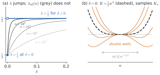
(a) \lambda jumps at \delta=0, while the effective exponent at finite n (grey) is smooth; (b) at \delta=0, samples of size n add a random quadratic term of size n^{-1/2} (drawn at zero and at one and two standard deviations either side).
What a finite sample does see is the effective exponent, the posterior mean excess loss in units of 1/n (Notebook 2 Exercise 2.3.2):
\lambda_{\rm eff}(n)=-\frac{d\log\bar Z_n}{d\log n}=n\,\mathbb E_{\pi_n}[K]\;\xrightarrow{\;n\to\infty\;}\;\lambda .
The posterior lives where the loss is below about 1/n. So the effective exponent reflects the shape of the loss at that height.
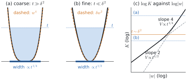
Above the loss level \delta^2 the loss looks quartic and its sublevel sets grow like t^{1/4} (a); below it they grow like t^{1/2} (b); on log-log axes (c) the local volume exponent is one over the slope.
With the prior roughly constant near 0, the effective exponent depends only on s=\delta\sqrt n (Exercise 3.1.2). It approaches \tfrac14 for small s and \tfrac12 for large s. The crossover is at n\sim\delta^{-2}, the sample size at which the data can detect the quadratic term.
Exercise 3.1 (The effective exponent).
- Compute \lambda for K=w^4+\delta w^2 at \delta=0 and at \delta>0, from V(t).
- With the prior constant near 0, rescale w=n^{-1/4}u to show \bar Z_n\approx\varphi(0)\,n^{-1/4}g(\delta\sqrt n) with g(s)=\int e^{-u^4-su^2}du, and from it derive \lambda_{\rm eff}=\tfrac14+\tfrac12\,s\,(-\log g)'(s). Show that \lambda_{\rm eff}\to\tfrac12 as s\to\infty.
- (Where \delta comes from.) Data: y=\varepsilon (noise of variance \sigma^2), x=(x_1,x_2) standard normal. Model f_w(x)=w^2x_1+\sqrt\delta\,w\,x_2 with loss \tfrac12(f_w(x)-y)^2. Show K=\tfrac12(w^4+\delta w^2). At \delta=0, show that the sample loss measured from w=0 is \tfrac12a_nw^4-u_nw^2 with a_n=1+O(n^{-1/2}) and u_n=O(\sigma n^{-1/2}). What does this say about detecting a \delta below n^{-1/2}?
Solution
1. At \delta=0, \{w^4<t\} is the interval |w|<t^{1/4}, so V\propto t^{1/4} and \lambda=\tfrac14. For \delta>0, near 0 the loss is \approx\delta w^2, so V\approx2\varphi(0)\sqrt{t/\delta} and \lambda=\tfrac12. The constant \propto\delta^{-1/2} blows up as \delta\to0: the limiting exponent jumps even though every finite-n integral varies continuously with \delta.
2. With w=n^{-1/4}u the exponent becomes u^4+\delta\sqrt n\,u^2 and dw=n^{-1/4}du, so \bar Z_n\approx\varphi(0)n^{-1/4}g(s). Since ds/d\log n=s/2,
\lambda_{\rm eff}=-\frac{d\log\bar Z_n}{d\log n}=\tfrac14-\tfrac s2(\log g)'(s)=\tfrac14+\tfrac s2(-\log g)'(s).
For large s the Gaussian factor confines u to |u|\lesssim s^{-1/2}, where u^4 is negligible. Then g\approx\sqrt{\pi/s}, (-\log g)'=1/2s, and \lambda_{\rm eff}\to\tfrac12. The crossover is at s\sim1.
3. Expand the square and average, using \mathbb Ex_i^2=1 and \mathbb E[x_1x_2]=\mathbb E[x_i\varepsilon]=0; the noise term \tfrac12\mathbb E\varepsilon^2 cancels against the minimum. At \delta=0 the sample replaces the averages by a_n=\overline{x_1^2} and u_n=\overline{x_1\varepsilon}, each a mean of n i.i.d. terms. So the sample loss has a quadratic term of random sign and size \sigma/\sqrt n: a double well when u_n>0, a steeper well otherwise. A true \delta below n^{-1/2} is lost in this noise, which is the s\lesssim1 regime of part 2.
Code. The effective exponent by quadrature for several \delta, against n and against \delta^2n, where the curves should collapse.
Code (19 lines)
w = np.linspace(-2, 2, 400_001)
dw = w[1] - w[0]
ns = np.logspace(0, 7, 57)
fig, ax = plt.subplots(1, 2, figsize=(9.5, 3.4))
for delta in [0.0, 0.003, 0.01, 0.03, 0.1, 0.3]:
    K = w**4 + delta * w**2
    lam_eff = []
    for n in ns:
        logp = -n * K
        p = np.exp(logp - logp.max()); p /= p.sum()
        lam_eff.append(n * (p * K).sum())
    lam_eff = np.array(lam_eff)
    ax[0].semilogx(ns, lam_eff, label=rf"$\delta={delta}$")
    if delta > 0:
        ax[1].semilogx(delta**2 * ns, lam_eff, label=rf"$\delta={delta}$")
for a in ax:
    a.axhline(0.25, color="k", ls=":"); a.axhline(0.5, color="k", ls=":"); a.set_ylabel(r"$\lambda_{\rm eff}(n)$")
ax[0].set_xlabel("n"); ax[0].legend(fontsize=8); ax[1].set_xlabel(r"$\delta^2 n$"); ax[1].set_title("the same curves against $\\delta^2 n$")
plt.tight_layout(); plt.show()
3.2 Sampling at temperature
Question: how do you measure the effective exponent when the loss is given only by data and gradients?
Notation: L_n mean training loss on n samples, \beta inverse temperature; w^* a minimizer of L_n in the basin of interest (in practice, the trained parameter); K_n=L_n-L_n(w^*); tempered posterior \propto\varphi e^{-\beta nL_n} with expectation \mathbb E_\beta; localizer strength \gamma, step size \epsilon, minibatch size b.
With a fixed data set you cannot vary n, but you can vary \beta. Differentiate in \beta instead of n (Notebook 1 Exercise 1.1.3), and assume the volume scaling of Notebook 2 with exponent \lambda:
-\partial_\beta\log\!\int\!\varphi e^{-\beta nK_n}=\mathbb E_\beta[nK_n]\approx\frac\lambda\beta, \qquad\text{so}\qquad \lambda\approx n\beta\big(\mathbb E_\beta[L_n]-L_n(w^*)\big).
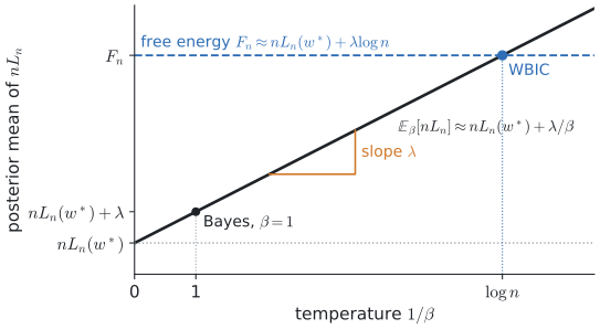
Schematically, the posterior mean of nL_n rises linearly in the temperature 1/\beta with slope \lambda; the estimator reads off the slope, and the value at 1/\beta=\log n is the WBIC.
- WBIC (Watanabe 2013). At \beta=1/\log n the posterior mean of nL_n is about nL_n(w^*)+\lambda\log n. Those are the leading terms of the free energy F_n=-\log\int\varphi e^{-nL_n}, obtained without knowing \lambda.
- Local learning coefficient (Lau et al. 2023). Read the other way, the formula estimates \lambda. A term \tfrac\gamma2\|w-w^*\|^2 added to the energy keeps the chain in the basin of w^*.
SGLD. The expectation is computed by stochastic gradient Langevin dynamics. It is gradient descent on the energy \beta nL_n+\tfrac\gamma2\|w-w^*\|^2, with a minibatch gradient \hat\nabla L_n and added Gaussian noise:
w\leftarrow w-\frac\epsilon2\Big(\beta n\,\hat\nabla L_n(w)+\gamma(w-w^*)\Big)+\sqrt\epsilon\,\xi, \qquad \xi\sim\mathcal N(0,I).
In the limit of small steps with full gradients, the chain’s stationary density is \propto e^{-\text{energy}}. With finite steps and minibatches it is biased and may not mix; it is used because each step costs one minibatch gradient. The estimate is n\beta times the gap between the chain’s average loss after burn-in and L_n(w^*).
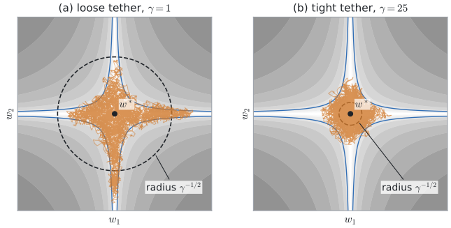
Langevin chains on K=(w_1w_2)^2 at n\beta=200: a loose tether (a) lets the chain run along the flat valley, a tight one (b) cuts the valley off and lowers the estimate from 0.37 to 0.12.
What the knobs do.
- \beta: the chain sits at excess loss \sim\lambda/(n\beta), so the estimate is the effective exponent at sample size n\beta, not \lambda. For w^4+\delta w^2 it moves from \tfrac14 to \tfrac12 as n\beta passes \delta^{-2}.
- \gamma: directions that stay flat beyond a distance \gamma^{-1/2} are cut off, which lowers the estimate (Exercise 3.2.3). The effect vanishes as n\beta\to\infty at fixed \gamma.
- \epsilon: the update is unstable unless \epsilon(n\beta\Lambda+\gamma)<4, with \Lambda the largest curvature of L_n the chain meets. Much smaller, and it does not mix.
- b: minibatch gradient noise acts as extra temperature.
Exercise 3.2 (The estimator).
- Derive \mathbb E_\beta[nK_n]\approx\lambda/\beta from the volume scaling, including the correction from a multiplicity m>1. Why does \beta=1/\log n give the free energy’s leading terms?
- (Predict before running.) Code 1 uses the model of Exercise 3.1.3 with n = 1000, σ = ½, δ = 0, 0.03 or 0.1, and β from 0.01 to 1. With K=\tfrac12(w^4+\delta w^2) and §3.1’s scaling at n\beta in place of n, predict where the estimate is near \tfrac14, near \tfrac12, or between. What does the sample noise of Exercise 3.1.3 do at \delta=0?
- (The localizer.) For a positive-definite quadratic basin in d parameters, with Hessian H of eigenvalues h_i and the Gaussian localizer, show \hat\lambda=\tfrac12\sum_i\frac{n\beta h_i}{n\beta h_i+\gamma}. Interpret it as a count of directions.
Hint
The chain samples a Gaussian with precision n\beta H+\gamma I.
Solution
1. Notebook 1 Exercise 1.1.3 with K_n for L_n gives the identity. With \int\varphi e^{-\beta nK_n}\approx c\,\Gamma(\lambda+1)(\beta n)^{-\lambda}(\log\beta n)^{m-1} (Notebook 2 §2.1 at \beta n),
\mathbb E_\beta[nK_n]=\frac\lambda\beta-\frac{m-1}{\beta\log(\beta n)} .
So for m=2 the estimate comes out low by a relative 1/\log(\beta n), which Code 2 shows. At \beta=1/\log n, \mathbb E_\beta[nL_n]=nL_n(w^*)+\mathbb E_\beta[nK_n]\approx nL_n(w^*)+\lambda\log n, the two leading terms of F_n. At \beta=1 the average is only \lambda above the minimum.
2. Rescaling u=(n\beta/2)^{1/4}w turns n\beta K into u^4+su^2 with s=\delta\sqrt{n\beta/2}, so the crossover is at n\beta\sim2/\delta^2. For δ = 0.1 that is nβ ≈ 200: β = 0.01 and 0.03 give about ¼, β = 0.1 is in between, and β = 0.3 and 1 move toward ½. For δ = 0.03 it is nβ ≈ 2200: about ¼ throughout, rising at β = 1. At \delta=0 the sample’s quadratic term (of size σ/√n ≈ 0.016) gives a regular minimum or a shallow double well, depending on its sign, with curvature comparable to δ ≈ 0.03. So at large \beta the \delta=0 estimate should also rise above \tfrac14.
3. Energy and localizer are both quadratic, so the chain samples \mathcal N\big(w^*,(n\beta H+\gamma I)^{-1}\big) and \mathbb E[nK_n]=\tfrac12\mathrm{tr}\big(nH(n\beta H+\gamma I)^{-1}\big). Multiply by \beta. Each direction counts \tfrac12 when its curvature n\beta h_i dominates \gamma and 0 when the localizer dominates. So the estimate is half the number of directions stiffer than the localizer: d/2 as \gamma\to0, and 0 as \gamma\to\infty.
Code 1. SGLD estimates (solid) against the exact tempered value on a grid (dashed), swept over \beta; compare with Exercise 3.2.2.
Code (31 lines)
n, batch, sigma = 1000, 100, 0.5
betas = np.array([0.01, 0.03, 0.1, 0.3, 1.0])
X = rng.standard_normal((n, 2))
y = sigma * rng.standard_normal(n)
w_grid = np.linspace(-1.5, 1.5, 60_001)

plt.figure(figsize=(6, 3.8))
for j, delta in enumerate([0.0, 0.03, 0.1]):
    def f(w, Xs): return w**2 * Xs[:, 0] + np.sqrt(delta) * w * Xs[:, 1]
    def loss_full(w): return 0.5 * np.mean((f(w, X) - y) ** 2)
    def grad_minibatch(w, idx):
        Xb, yb = X[idx], y[idx]
        return np.mean((f(w, Xb) - yb) * (2 * w * Xb[:, 0] + np.sqrt(delta) * Xb[:, 1]))
    L_grid = 0.5 * np.mean((w_grid[:, None] ** 2 * X[None, :, 0] + np.sqrt(delta) * w_grid[:, None] * X[None, :, 1] - y[None, :]) ** 2, axis=1)
    w_star = w_grid[np.argmin(L_grid)]
    exact, sgld = [], []
    for beta in betas:
        logp = -n * beta * L_grid
        p = np.exp(logp - logp.max()); p /= p.sum()
        exact.append(n * beta * ((p * L_grid).sum() - L_grid.min()))
        est = sgld_lambda(grad_minibatch, loss_full, np.array(w_star), n, batch, n * beta, gamma=1.0,
                          eps=1e-3, steps=12000, burn=2000, chains=3)
        sgld.append(est)
    sgld = np.array(sgld)
    plt.errorbar(n * betas, sgld.mean(1), sgld.std(1), fmt="o-", color=f"C{j}", capsize=3, label=rf"SGLD, $\delta={delta}$ ($w^*={w_star:.2f}$)")
    plt.plot(n * betas, exact, "--", color=f"C{j}", label=rf"exact tempered mean, $\delta={delta}$")
for d in [0.03, 0.1]:
    plt.axvline(2 / d**2, color="k", ls=":", lw=0.8)
plt.axhline(0.25, color="k", ls=":"); plt.axhline(0.5, color="k", ls=":")
plt.xscale("log"); plt.xlabel(r"$n\beta$"); plt.ylabel(r"$\hat\lambda$"); plt.legend(fontsize=7, ncol=2)
plt.title(r"$K=\frac{1}{2}(w^4+\delta w^2)$ from data, $n=1000$; dotted: $n\beta=2/\delta^2$"); plt.tight_layout(); plt.show()
Code 2: normal crossings. f_w(x)=w_1^aw_2^bx fitting noise (as in Lau et al., Table 1), where \lambda=\min(\tfrac1{2a},\tfrac1{2b}), with m=2 when a=b (Notebook 2 Exercise 2.2.2); SGLD against the exact localized value.
Code (24 lines)
n, batch = 1000, 100
nbeta = n / np.log(n)
Xc = rng.standard_normal(n)
yc = 0.25 * rng.standard_normal(n)
g1 = np.linspace(-2, 2, 801)
W1, W2 = np.meshgrid(g1, g1, indexing="ij")
sx2, sxy = np.mean(Xc**2), np.mean(Xc * yc)
print(f"{'(a,b)':8s} {'lambda':>7s} {'exact tempered':>15s} {'SGLD (3 chains)':>22s}")
for (a, b) in [(1, 1), (1, 2), (1, 3), (2, 2)]:
    lam = min(1 / (2 * a), 1 / (2 * b))
    def f(w, Xs): return w[0]**a * w[1]**b * Xs
    def loss_full(w): return 0.5 * np.mean((f(w, Xc) - yc) ** 2)
    def grad_minibatch(w, idx):
        Xb, yb = Xc[idx], yc[idx]; r = f(w, Xb) - yb
        return np.array([np.mean(r * Xb * a * w[0]**(a - 1) * w[1]**b), np.mean(r * Xb * b * w[0]**a * w[1]**(b - 1))])
    w_star = np.zeros(2)
    # exact: L_n(w) = 1/2 c^2 mean(x^2) - c mean(x y) + 1/2 mean(y^2), with c = w1^a w2^b
    C = W1**a * W2**b
    L_grid = 0.5 * C**2 * sx2 - C * sxy + 0.5 * np.mean(yc**2)
    logp = -nbeta * L_grid - 0.5 * 1.0 * (W1**2 + W2**2)
    p = np.exp(logp - logp.max()); p /= p.sum()
    exact = nbeta * ((p * L_grid).sum() - loss_full(w_star))
    est = sgld_lambda(grad_minibatch, loss_full, w_star, n, batch, nbeta, gamma=1.0, eps=1e-3, steps=10000, burn=2000, chains=3)
    print(f"({a},{b})    {lam:7.3f} {exact:15.3f} {est.mean():12.3f} +- {est.std():.3f}")
(a,b) lambda exact tempered SGLD (3 chains) (1,1) 0.500 0.344 0.386 +- 0.017 (1,2) 0.250 0.200 0.219 +- 0.045 (1,3) 0.167 0.136 0.139 +- 0.055 (2,2) 0.250 0.147 0.162 +- 0.042
Code 3: a two-layer linear network. f(x)=BAx with 3\times3 matrices (d=18) and a rank-r teacher, whose \lambda Aoyagi and Watanabe (2005) computed; then the estimate as the localizer tightens.
n, batch, m_dim = 1000, 100, 3
nbeta = n / np.log(n)
X3 = rng.standard_normal((n, m_dim))

def aoyagi_watanabe(m, r):
    return (m + r) * (3 * m - r) / 8 + (1 / 8 if (m + r) % 2 else 0.0)

def make_problem(r):
    s = np.zeros(m_dim); s[:r] = 1.0
    A0 = np.diag(np.sqrt(s)); B0 = np.diag(np.sqrt(s))
    Y = X3 @ (B0 @ A0).T + 0.1 * rng.standard_normal((n, m_dim))
    def unpack(w): return w[:9].reshape(3, 3), w[9:].reshape(3, 3)
    def loss_full(w):
        A, B = unpack(w); R = X3 @ (B @ A).T - Y
        return 0.5 * np.mean(np.sum(R**2, 1))
    def grad_minibatch(w, idx):
        A, B = unpack(w); Xb, Yb = X3[idx], Y[idx]
        R = Xb @ (B @ A).T - Yb
        return np.concatenate([(B.T @ R.T @ Xb / len(idx)).ravel(), (R.T @ Xb @ A.T / len(idx)).ravel()])
    w = np.concatenate([A0.ravel(), B0.ravel()])
    for _ in range(2000):                      # gradient descent to the sample's minimizer near the teacher
        w = w - 0.05 * grad_minibatch(w, np.arange(n))
    return loss_full, grad_minibatch, w

# TODO: for r in 3, 2, 1, 0 estimate lambda with sgld_lambda(..., nbeta, gamma=1.0, eps=3e-4, steps=6000, burn=1000)
#       and print it next to aoyagi_watanabe(3, r); then sweep gamma over [0.3, 1, 3, 10, 30, 100] at r = 3.
Solution (code)
n, batch, m_dim = 1000, 100, 3
nbeta = n / np.log(n)
X3 = rng.standard_normal((n, m_dim))

def aoyagi_watanabe(m, r):
    return (m + r) * (3 * m - r) / 8 + (1 / 8 if (m + r) % 2 else 0.0)

def make_problem(r):
    s = np.zeros(m_dim); s[:r] = 1.0
    A0 = np.diag(np.sqrt(s)); B0 = np.diag(np.sqrt(s))
    Y = X3 @ (B0 @ A0).T + 0.1 * rng.standard_normal((n, m_dim))
    def unpack(w): return w[:9].reshape(3, 3), w[9:].reshape(3, 3)
    def loss_full(w):
        A, B = unpack(w); R = X3 @ (B @ A).T - Y
        return 0.5 * np.mean(np.sum(R**2, 1))
    def grad_minibatch(w, idx):
        A, B = unpack(w); Xb, Yb = X3[idx], Y[idx]
        R = Xb @ (B @ A).T - Yb
        return np.concatenate([(B.T @ R.T @ Xb / len(idx)).ravel(), (R.T @ Xb @ A.T / len(idx)).ravel()])
    w = np.concatenate([A0.ravel(), B0.ravel()])
    for _ in range(2000):                      # gradient descent to the sample's minimizer near the teacher
        w = w - 0.05 * grad_minibatch(w, np.arange(n))
    return loss_full, grad_minibatch, w

print(f"{'rank r':>6s} {'lambda (Aoyagi-Watanabe)':>26s} {'SGLD estimate':>22s}     (d/2 = 9)")
for r in [3, 2, 1, 0]:
    loss_full, grad_minibatch, w_star = make_problem(r)
    est = sgld_lambda(grad_minibatch, loss_full, w_star, n, batch, nbeta, gamma=1.0, eps=3e-4, steps=6000, burn=1000, chains=3)
    print(f"{r:6d} {aoyagi_watanabe(3, r):26.3f} {est.mean():14.2f} +- {est.std():.2f}")

loss_full, grad_minibatch, w_star = make_problem(3)
gammas = [0.3, 1, 3, 10, 30, 100]
sweep = np.array([sgld_lambda(grad_minibatch, loss_full, w_star, n, batch, nbeta, gamma=g, eps=3e-4, steps=6000, burn=1000, chains=3) for g in gammas])
plt.figure(figsize=(5, 3.3))
plt.errorbar(gammas, sweep.mean(1), sweep.std(1), fmt="o-", capsize=3)
plt.axhline(aoyagi_watanabe(3, 3), color="k", ls=":", label=r"$\lambda=4.5$"); plt.axhline(9, color="k", ls="--", lw=0.8, label=r"$d/2=9$")
plt.xscale("log"); plt.xlabel(r"localization $\gamma$"); plt.ylabel(r"$\hat\lambda$"); plt.title("rank-3 teacher: the estimate against the localizer")
plt.legend(); plt.tight_layout(); plt.show()
rank r lambda (Aoyagi-Watanabe) SGLD estimate (d/2 = 9)
3 4.500 4.70 +- 0.13
2 4.500 4.48 +- 0.09
1 4.000 3.93 +- 0.14
0 3.500 3.34 +- 0.12
