Training dynamics · Lecture 2

The pragmatic picture

What the knobs of a training run do, and which derivation stands behind each one

learning rate · batch size · schedule · optimizer · width · normalization and weight decay · what they act on

About 15 minutes. Nothing is derived on the board: every result on these slides is an exercise with a worked solution in the notebook named at the bottom of the slide. The longer outline, with timings and the full speaker notes, is L2_pragmatic_picture.md. Keys: N toggles these notes, S opens the speaker view.

Notation on the board (matches NB2): loss $L$, gradient $g=\nabla L$, Hessian $H$, sharpness $S=\lambda_{\max}(H)$, step $\eta$, batch size $B$, per-example gradient covariance $\Sigma$. Time is $t=k\eta$, so gradient flow is $\dot\theta=-\nabla L$.

Symbol clashes to warn about once: $\Sigma$ is the target correlation in NB1 and the noise covariance here; $\lambda$ is a Hessian eigenvalue in td2_1/td2_2, the NTK in the catapult, and the weight decay in td2_5; $P$ is Adam's preconditioner in td2_2–td2_5 and the parameter count in td2_6.

Two kinds of tools, one picture

1. Small-step expansions. Treat training as a flow plus corrections, or as a stochastic differential equation. The expansion parameter is $\eta S$. These give the scaling rules.

2. Where they break. Real training sits at $\eta S\approx2$, exactly where "small step" fails, and different tools take over.

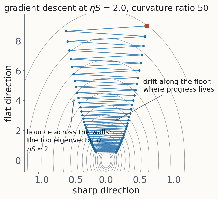
Keep this valley on the board. The bounce across the walls is the top eigenvector; progress is the drift along the floor. Segments on the learning rate, the schedule, curvature and what is learned first all come back to it.

Gradient descent at eta S = 2 bouncing across a narrow valley while drifting along its floor

§1 · Learning rate as a step size

Gradient descent follows a modified flow that penalizes the gradient norm

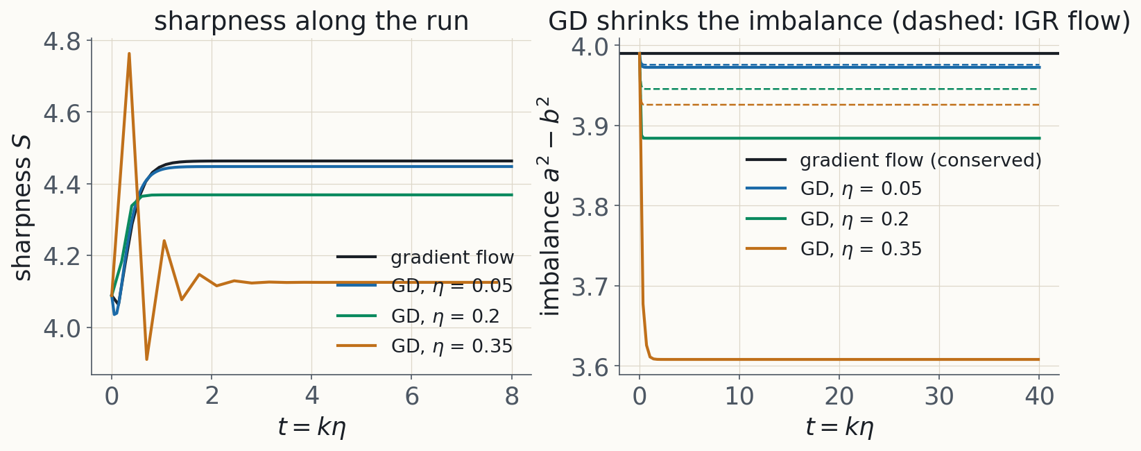
$$\dot\theta=-\nabla\Big(L+\tfrac{\eta}{4}\|\nabla L\|^2\Big)$$

On a quadratic, GD converges iff $\eta S<2$.
GD's gradient doesn't shrink along a step, so each step overshoots by $-\tfrac{\eta^2}{2}Hg$. As a drift, that is the penalty: implicit gradient regularization.
Asymptotic series. Degrades smoothly as $\eta S$ grows; no flow at all once $\eta\lambda\ge1$ in some direction.
Momentum: effective step $\eta/(1-\beta)$, edge $2(1+\beta)/\eta$.

GD, gradient flow and the IGR flow on L = (ab-1)^2/2: sharpness along the run and the layer imbalance

$L=\tfrac12(ab-1)^2$ from $(2,0.1)$. Gradient flow conserves $a^2-b^2$; GD shrinks it, and the IGR flow (dashed) accounts for 81%, 42% and 16% of the shift at $\eta S\approx0.2$, $0.8$, $1.4$.

td2_1_flows §1.1–1.3 (Barrett & Dherin), §1.5 momentum (Goh's Distill article)

§2 · Batch size

To first order, SGD is gradient flow plus noise of strength $\eta/B$

$$d\theta=-\nabla L\,dt+\sqrt{\tfrac{\eta}{B}}\,\Sigma^{1/2}dW$$

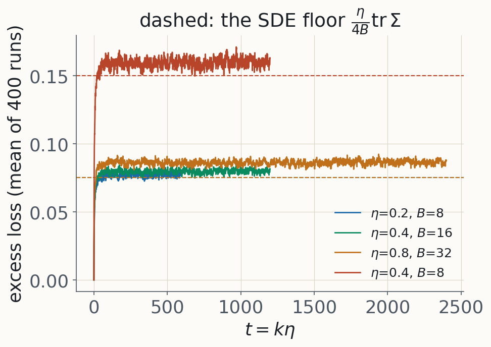
Holding $\eta/B$ fixed holds the SDE fixed: the linear scaling rule.
In a basin the floor is $\tfrac{\eta}{4B}\mathrm{tr}\,\Sigma$, with no $H$ in it.
A one-step Taylor model gives the critical batch $B_{\rm noise}=\mathrm{tr}(H\Sigma)/(g^\top Hg)$, past which larger batches buy almost nothing.
Adam: temperature $\eta/\sqrt B$, hence a square-root rule.

Excess loss of SGD on a quadratic for three runs with the same eta/B and one with twice it

Diagonal quadratic, Gaussian gradient noise. Same $\eta/B$, same floor, until $\eta h$ stops being small in the top mode ($\eta=0.8$ sits above the line).

td2_2_sgd_sde §2.1–2.6 (Li, Malladi & Arora; McCandlish et al.; Malladi et al.), §2.7 validity

The order-2 stochastic modified equation adds IGR's drift $\tfrac\eta4\|\nabla L\|^2$, which depends on $\eta$, not $\eta/B$, so the linear scaling rule is a first-order statement. It fails once $B$ approaches $B_{\rm noise}$, when $\eta h$ isn't small in the top directions (the orange run), and at the edge of stability. $\Delta L_{\rm opt}(B)=\Delta L_{\max}/(1+B_{\rm noise}/B)$.

Adam's rule, stated only: under $B\to\kappa B$, take $\eta\to\sqrt\kappa\eta$, $1-\beta_i\to\kappa(1-\beta_i)$, $\epsilon\to\epsilon/\sqrt\kappa$. Needs noise-dominated gradients.

Competing accounts, present evenly. What does the noise buy? One view: the temperature $\eta/B$ is the important parameter. Smith, Dherin, Barrett and De: the finite-$\eta$ drift corrections matter more for generalization (§2.7 item 4). Is the noise Gaussian? Şimşekli et al. argue heavy tails; Li, Malladi and Arora find matched-covariance Gaussian noise reaches the same CIFAR-10 accuracy (§2.7 item 7). "Is the Taylor expansion even valid?" §2.7 collects nine answers; weak-order bounds hold on a fixed horizon as $\eta\to0$ and nothing quantitative follows for a given $\eta$. Testable with SVAG (§2.5).

Picked up in: td2_2 §2.2 (the SDE), §2.3 (the floor), critical batch, scaling rules, validity.

§3 · Where the expansions break: the edge of stability

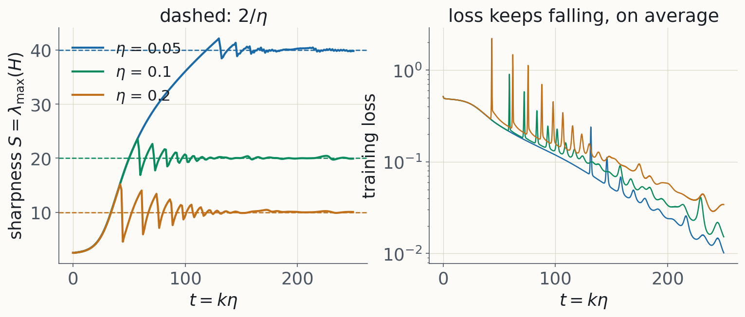
Sharpness rises to $2/\eta$ and stays there while the loss keeps falling

Sharpness of a small MLP under full-batch GD at three step sizes, each rising to its own 2/eta, and the loss

$$\nabla L(\bar\theta+xu)=\nabla L(\bar\theta)+xSu+\tfrac12x^2\nabla S+O(x^3)$$

Tanh MLP, 256 random labels, full-batch GD. All three runs follow the same curve in $t=k\eta$ until each hits its own $2/\eta$. The $x^2$ term survives the period-2 average: self-stabilization.

td2_3_edge_of_stability §3.1–3.4 (Cohen et al.; Damian, Nichani & Lee; central flows, Rod Flow)

This is exactly where the expansion of the previous slide fails. The bounce across the valley is the oscillation along $u$; the $\tfrac12x^2\nabla S$ push moves the iterate toward lower walls.

The central flow models the time-averaged trajectory: $dw/dt=-[\nabla L+\tfrac12\sigma^2\nabla S]$, with $\sigma^2$ fixed by requiring $S$ to stay at $2/\eta$; its time-averaged loss is $L+\sigma^2/\eta$. State it, don't derive it (Exercise 3.3). Heuristic, and Cohen et al. state its limits. Rod Flow tracks the midpoint and half-length of consecutive iterates; principal flow resums the backward-error terms built from $H$ and captures the onset but not the stabilization (§3.4).

Open question to name: why progressive sharpening happens is only partly understood. td2_3 takes it as given.

Under SGD the quantity at $2/\eta$ is a batch sharpness and the full-batch $S$ settles lower (§3.6). Adam holds a preconditioned sharpness at $38/\eta$ at $\beta_1=0.9$ (§3.5).

Show, if time: eos_toy_and_catapult.html, panel 1, preset "EoS from below". Picked up in: td2_3 §3.1 (this figure).

§3 · Where the expansions break: the catapult

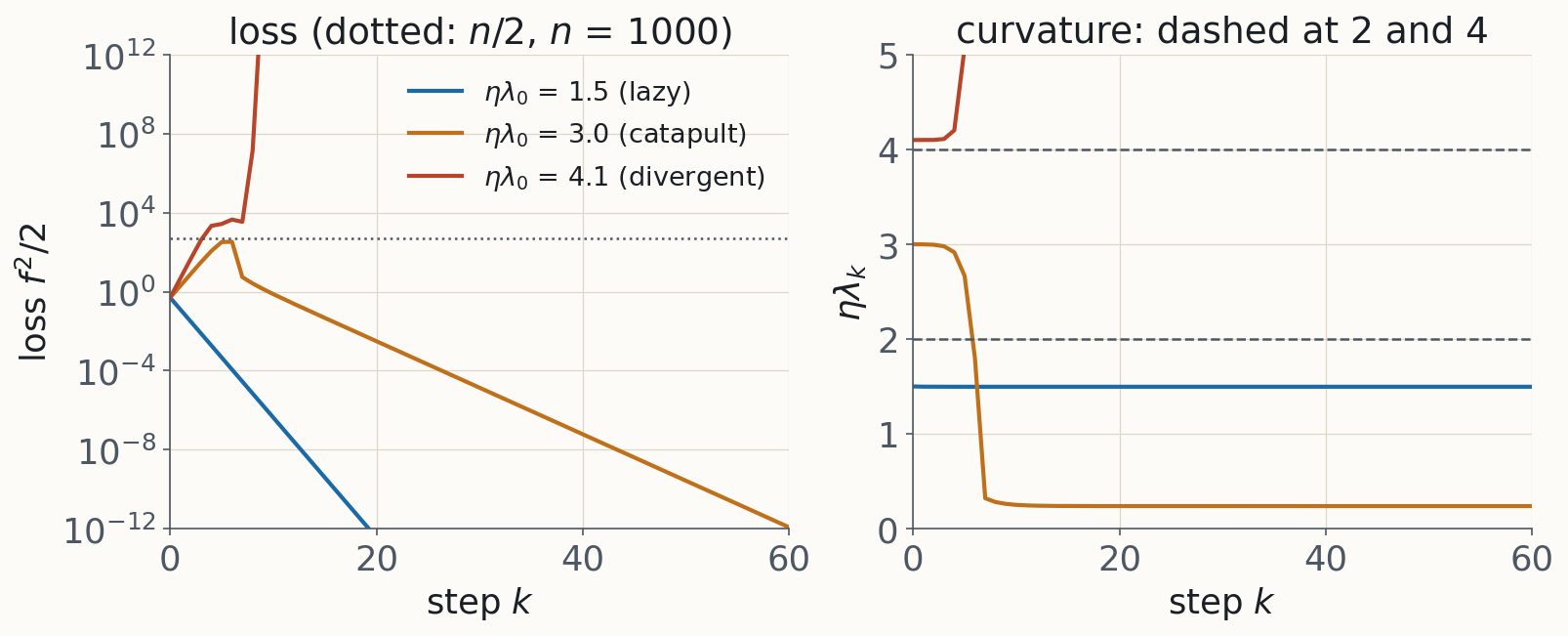
A large step can lower the curvature in one shot

The exact catapult maps at eta lambda_0 = 1.5, 3 and 4.1: loss and curvature against step

Width-$n$ two-layer net, one input, exact maps. $\eta\lambda_0<2$ lazy; $2<\eta\lambda_0<4$ the loss spikes, the curvature drops, training converges somewhere flatter; $\eta\lambda_0>4$ diverges.

Contrast with the edge of stability: self-stabilization is a sustained hover, the catapult a one-shot drop with nothing pushing the curvature back up.
The $4/\lambda_0$ edge is specific to this model; ReLU nets in the paper tolerate up to about $12/\lambda_0$.

td2_3_edge_of_stability §3.7 (Lewkowycz et al.)

§4 · Schedule

Both ends of a schedule have a mechanism, and each end has more than one

Warmup. Edge-of-stability account: starting at the target $\eta$ from a sharp initialization catapults or diverges; ramping lets $S$ follow $2/\eta(t)$ down. Adam account: early $\hat v$ is estimated from few samples, so the adaptive step has high variance.

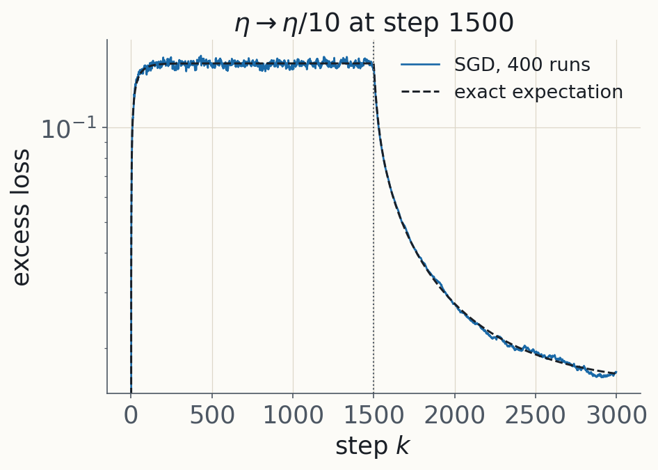
Decay. Three pictures of one observation, that the loss drops when $\eta$ is cut: the fluctuation floor $\tfrac{\eta}{4B}\mathrm{tr}\,\Sigma$; Wen et al.'s river valley, where noise bounces the iterate between the hillsides and hides progress along the river; an edge-of-stability analogue, where the measured loss is $L+\sigma^2/\eta$.

Excess loss of SGD before and after the learning rate is cut tenfold, against the exact expectation

Same quadratic. The dashed line is the exact expectation, not a fit. The target drops tenfold at once; the loss follows mode by mode at rates $2\eta'h_j$.

td2_3_edge_of_stability §3.8 (Kalra & Barkeshli; Wen et al.) · td2_2_sgd_sde §2.3

§5 · Optimizer

An optimizer has to decide what counts as a small step. That decision is a norm.

$$\Delta=\arg\min_{\|\Delta\|\le\eta}\langle g,\Delta\rangle=-\eta\,d^\star(g),\qquad d^\star(g)\in\arg\max_{\|d\|\le1}\langle g,d\rangle$$

Steepest descent under the Euclidean, l-infinity and an M-norm: unit balls with the step at the supporting line

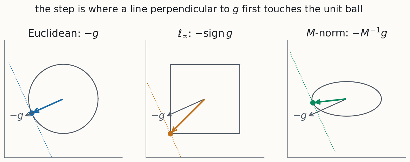
Euclidean: GD. $\ell_\infty$: sign descent (Adam with its averages off). Fisher norm: natural gradient. Spectral norm on a weight matrix: $UV^\top$, which Muon approximates by Newton–Schulz.
Every optimizer is steepest descent under some norm, so the dictionary explains nothing on its own. A norm earns its place by parametrization invariance or by step sizes that transfer across width.

td2_4_optimizer_geometry §4.0–4.4 (Bernstein & Newhouse; Martens; Jordan et al.)

The parable, labelled as an analogy as td2_4 §4.0 does: between point masses with disjoint supports, KL is infinite and Jensen–Shannon constant, so neither gives a gradient; Wasserstein-1 is $|\theta|$ because only it uses the geometry of the space. The parameter-space version is only the question "in which geometry should a step be measured?" The GAN theorems imply nothing about optimizers.

Natural gradient is invariant to reparametrization to first order. Raw sharpness is not: the Hessian is a quadratic form and its eigenvalues need a metric. This links to the MDL day's flatness discussion (Dinh et al.).

Adam's edge: with a frozen preconditioner, Adam at $\beta_1=0.9$ is stable iff $\eta\lambda_{\max}(P^{-1}H)<38$ (td2_3 §3.5). "Adam is sign descent" is exact only with the averages off (§4.3.D gives the failures). The squared-penalty form of the problem points the same way as the trust-region form, with a step $\|g\|_*$ times longer.

Show, if time: steepest_descent_balls.html, and try $g_2\approx0$ to see why sign descent is sensitive to small gradient components. Picked up in: td2_4 §4.1, §4.2 natural gradient, §4.3 Adam, §4.4 Muon.

§6 · Width

Which step sizes transfer across width? A spectral condition answers, and gives muP

$$\|W_l\|_2=\Theta\Big(\sqrt{\tfrac{n_l}{n_{l-1}}}\Big),\quad\|\Delta W_l\|_2=\Theta\Big(\sqrt{\tfrac{n_l}{n_{l-1}}}\Big)$$

Gradient updates are low-rank and aligned with the incoming features, so their spectral norm measures their effect on the activations.
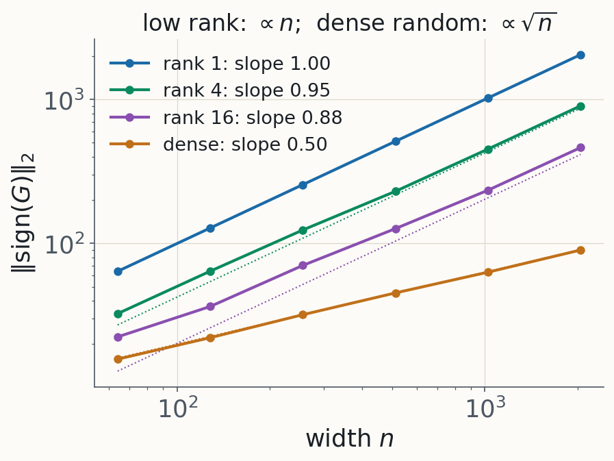
For low-rank $G$, $\|\mathrm{sign}(G)\|_2=\Theta(\sqrt{n_ln_{l-1}})$, so Adam needs $\eta_l=\Theta(1/\text{fan-in})$: muP's rule. Muon's $\|UV^\top\|_2=1$ gives $\eta_l=\Theta(\sqrt{n_l/n_{l-1}})$ directly.
A dense random sign matrix would give only $\Theta(\sqrt n)$: the structure of the gradient sets the exponent.

Spectral norm of sign(G) against width for low-rank and dense random G

$\|\mathrm{sign}(G)\|_2$ against width, $G$ of rank 1, 4, 16 and dense Gaussian. Dotted: $\mathbb E|w_1|\,n$ and $2\sqrt n$.

td2_4_optimizer_geometry §4.5 (Yang, Simon & Bernstein), §4.6 the modular norm

§7 · Normalization and weight decay

Behind a normalization layer the loss sees only a direction. Weight decay sets the step it takes.

$$\langle\nabla L(w),w\rangle=0,\ \ \eta_{\rm eff}\approx\frac{\eta}{\|w\|^2};\qquad\cos\theta^*=1-\eta\lambda$$

The gradient is tangent, so a step lengthens $w$ by Pythagoras; without decay the norm only grows and the effective step decays like $1/\sqrt k$.
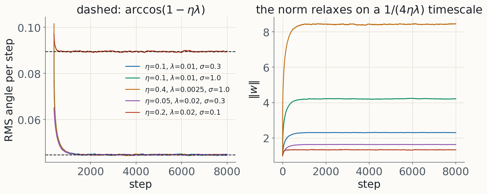
Weight decay pulls radially in. At equilibrium each block rotates by a fixed angle $\theta^*\approx\sqrt{2\eta\lambda}$ per step, whatever its gradient scale.
On scale-invariant weights, weight decay is a learning-rate schedule, not a regularizer of the function. Li & Arora: exactly equivalent to an exponentially increasing $\eta$.

RMS rotation angle per step and weight norm for five (eta, lambda, sigma) settings on a scale-invariant toy; settings with the same eta*lambda reach the same angle

Noisy scale-invariant toy, SGD. Four settings share $\eta\lambda=10^{-3}$ and end at the same angle; the norm relaxes on a $1/(4\eta\lambda)$ timescale, often a sizeable part of a schedule.

td2_5_normalization_weight_decay §5.1–5.2 (Kosson et al.; Li & Arora; D'Angelo et al.)

§7 · Loss spikes and clipping

Four documented spike mechanisms, sorted by whether they are an edge-of-stability crossing

Mechanism	Edge crossing?	Fix
Weight decay shrinks a normalized layer until $\eta_{\rm eff}S$ crosses 2	yes	schedule $\eta\lambda$; watch $\\|w\\|$
Adam's second moment goes stale, so the preconditioned sharpness crosses $38/\eta$	yes	$\beta_2$, $\epsilon$ (Bai et al.; Molybog et al.)
Attention-logit growth	no	QK-layernorm
Output-logit drift along a flat direction	no	z-loss

Clipping. Under $(L_0,L_1)$-smoothness, where curvature grows with the gradient norm, the right step is $\propto1/\|\nabla L\|$ where the gradient is large. That is clipping.

td2_5_normalization_weight_decay §5.3 spikes, §5.4 clipping (Zhang et al.)

§8 · What the knobs act on: curvature

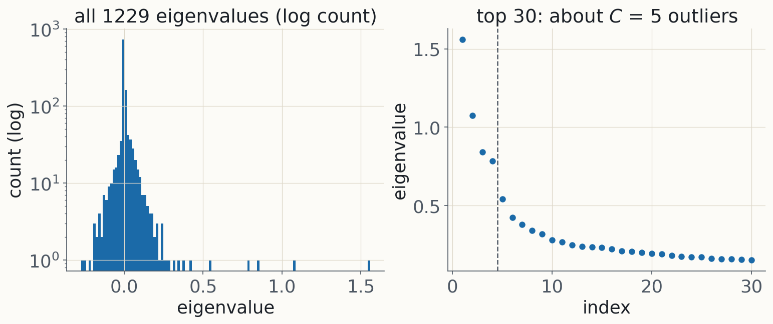
The Hessian is a bulk at zero plus about $C$ outliers. The gradient lives in the outliers; progress mostly doesn't.

Hessian spectrum of a small five-class classifier: a bulk at zero and about five outliers

GELU MLP, 1229 parameters, $C=5$ Gaussian classes, cross-entropy, stopped at loss 0.24. Full eigh.

$H$ = Gauss–Newton + residual. The Gauss–Newton part shares its nonzero spectrum with the loss-weighted tangent kernel, so progressive sharpening with square loss is the kernel moving.
The outliers are tied to class means of gradients.
A step along a direction of curvature $\lambda$ gains $\Delta L=-\eta g^2(1-\eta\lambda/2)$: at the edge the gain cancels. The top subspace is the bounce; the drift along the floor lives in the bulk.
The basin is chosen early, when the kernel moves fastest.

td2_6_curvature §6.1–6.5 (Sagun et al.; Papyan; Song, Ahn & Yun; Fort et al.; Frankle et al.)

§8 · What the knobs act on: order of learning

Low-order statistics first, then the rest, at a sample cost set by where the signal hides

Moments before cumulants. A model linear in its inputs sees only the first two moments, so a network with small pre-activations learns from Gaussian-equivalent statistics first. Train on the data and on its Gaussian clone: the early curves coincide.
The price of a hidden direction. A direction visible only in the $k$-th cumulant costs about $d^{\,k-1}$ samples for information exponent $k\ge3$, far fewer if it correlates with lower-order structure.
Spectral bias. A fixed kernel fits eigenfunction $k$ at rate $\lambda_k$: low frequencies first.

If L1 was skipped: shallow, $\dot a=s-a$; two-layer from small balanced init, $\dot a=2a(s-a)$, so the strongest structure first, after a plateau.

td2_7_learned_first §7.1–7.3 (Refinetti et al.; Bardone & Goldt; Basri et al.)

§9 · Menu

Pick a knob. Each notebook stands alone, opens with its readings, and the derivations follow.

Knob or question	Notebook	Core reading
Learning rate as a step size: flows, IGR, momentum	td2_1_flows	Barrett & Dherin
Batch size: SMEs, loss floor, critical batch, linear and square-root rules, validity	td2_2_sgd_sde	Li, Malladi & Arora
Where the expansions break: EoS, central flows, Adam's and SGD's edges, catapult, warmup and WSD	td2_3_edge_of_stability	Cohen et al.
Optimizer and width: norms, natural gradient, Adam as sign descent, Muon, muP	td2_4_optimizer_geometry	Bernstein & Newhouse
Normalization, weight decay, spikes, clipping	td2_5_normalization_weight_decay	Kosson et al.
What the Hessian looks like; when the basin is chosen	td2_6_curvature	Song, Ahn & Yun
What is learned first	td2_7_learned_first	Refinetti et al.
Dropout, layer cushion, geometry-adaptive bases, critical periods, RL fine-tuning dynamics	td2_8_further_readings	readings with short exercises

§9 · Routes

Three ways through the afternoon

Less background. NB1 §1, §4 and §5 (mode equations, the kernel, lazy versus rich), then td2_1 and td2_2. Flows and SDEs are one story: backward error analysis, first for the step and then in distribution.
Practitioner-minded. td2_2 → td2_4 → td2_5: batch size, optimizer, normalization and weight decay.
More background. Skim NB1, then any NB2 notebook. td2_3 and td2_6 are where the expansions break and the empirical phenomenology lives.

Out of scope today: whether SGD samples a Bayesian posterior (MDL day, WB2 §8); infinite-width NTK theory (Physics of Deep Learning day); measuring curvature at scale (DA day, L2).

(Room for the instructor's own recommendations.)