Data attribution · Lecture 1

What did this training example do?

From a causal question to one formula, and what that formula actually answers

The question

Which training examples made the model do this?

An example

Which pretraining texts make this response likely?

Query: a dialogue in which an AI assistant says it does not consent to being shut down.

810M model: top sequences

Share words with the query ("continue", "existing"), but not its meaning.

52B model: top sequences

Are about wanting to keep existing: an AI pleading with its crew; a person surviving in a desert.

The framing

Causal analysis of a training run

interpretability

input

→

layers

→

output

data attribution

training data

→

optimizer steps

→

weights

→

behaviour

Ablating a layer costs a forward pass. Ablating an example costs a training run.

The plan

One question, one formula, and what it answers

1 · Counterfactuals are subtle

2 · Data weights make deletion differentiable

3 · Derive the influence function; test it on regression

4 · What breaks for networks, and what the fixes answer

5 · How to check an attribution

6 · Another $\pi$: the training run, and a map of the afternoon

§1 · Counterfactuals

"Example $i$ caused it if deleting $i$ and retraining changes it."

What could go wrong?

§1 · Overdetermination

Two causes, each sufficient

butter	yeast	croissants
premium	premium	fluffy
standard	premium	fluffy
premium	standard	fluffy
standard	standard	flat

Leave-one-out credits neither. In training: a behaviour taught by many redundant examples.

The bakery: premium butter makes more steam, premium yeast makes more gas, and either alone is enough for fluffy croissants. Downgrading only one changes nothing, so LOO says neither caused the fluffiness, though both did.

Picked up in: DA1 §1 (Mueller 2024 is the reading, §4; written about interpretability, and the same failures apply).

Non-transitivity (cut from the slides; tell it if there is time): a boulder falls toward a hiker, she ducks, she survives. Ducking depends on the boulder and survival on ducking, but survival does not depend on the boulder: without it she survives anyway. Dependence does not chain (Ned Hall's example, as told by Hitchcock 2001; Mueller 2024 §3). In training: an example can be necessary for a feature that a capability uses, yet deleting it changes no output.

§1 · Shapley values

Average over every subset the example could join

$$\varphi_i=\mathbb E_{\text{random order}}\big[v(S\cup\{i\})-v(S)\big],\quad S=\text{examples before }i$$

Croissants: butter $\tfrac12$, yeast $\tfrac12$. The price: each $v(S)$ is a retraining, for up to $2^{n-1}$ subsets.

$v(S)$: the behaviour of a model trained on subset $S$. Shuffle the $n$ examples uniformly at random and add them one by one; $\varphi_i$ is the expected jump in $v$ when $i$ arrives. Equivalently (DA1 §1), $\varphi_i=\frac1n\sum_{S\subseteq[n]\setminus\{i\}}\binom{n-1}{|S|}^{-1}[v(S\cup\{i\})-v(S)]$: average over subsets of each size, then over the sizes. In the bakery $v(S)=1$ if $S$ contains butter or yeast; LOO gives 0 to everything, Shapley gives butter and yeast ½ each, flour and sugar 0.

Shapley attributes over finite coalitions: it is not the derivative at the full training set that the rest of the day computes. Practical versions sample permutations (Ghorbani & Zou 2019). It still splits credit between sufficient causes, where one could argue each deserves all of it.

§1 · Takeaway

"The influence of example $i$" is ambiguous until you say which counterfactual.

§2 · The formalism

How do you make "delete example $i$" something you can differentiate?

§2 · Data weights

Give every example a weight

$$L(w;\beta)=\sum_{i=1}^n\beta_i\,L_i(w)$$

$\beta=\mathbf 1$ is the real run; $\beta_i:1\to0$ deletes example $i$.

§2 · The object of study

Weights → trained model → behaviour

$$\beta\;\xrightarrow{\ \ \pi\ \ }\;\pi(\beta)\;\xrightarrow{\ \ \phi\ \ }\;\phi\big(\pi(\beta)\big)$$

$\pi$, "the trained model", is a modelling choice. $\phi$ is the behaviour: a test loss, a logit.

§2 · Influence

The influence of example $i$ on $\phi$

$$\mathcal I_i=\frac{\partial\,\phi(\pi(\beta))}{\partial\beta_i}\bigg|_{\beta=\mathbf 1}$$

Deleting $i$ changes $\phi$ by about $-\mathcal I_i$. On a test loss, a helpful example has $\mathcal I_i<0$.

§2 · Three targets

Three questions, at three distances from the real run

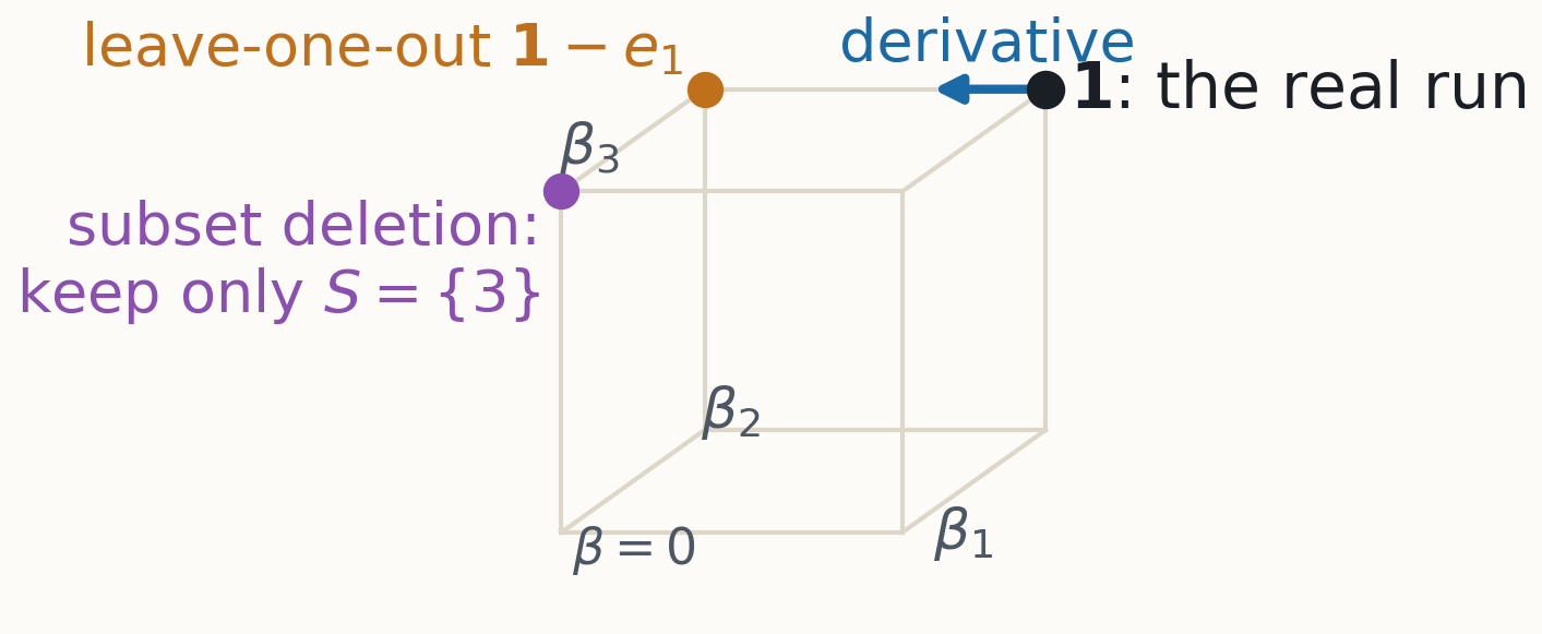
The cube of data weights for three examples: the real run at the all-ones corner, a derivative arrow, the leave-one-out corner one edge away, and a subset-deletion corner two edges away

The derivative; leave-one-out; deleting a large random subset.

§2 · A puzzle for later

The derivative and the deletion can disagree

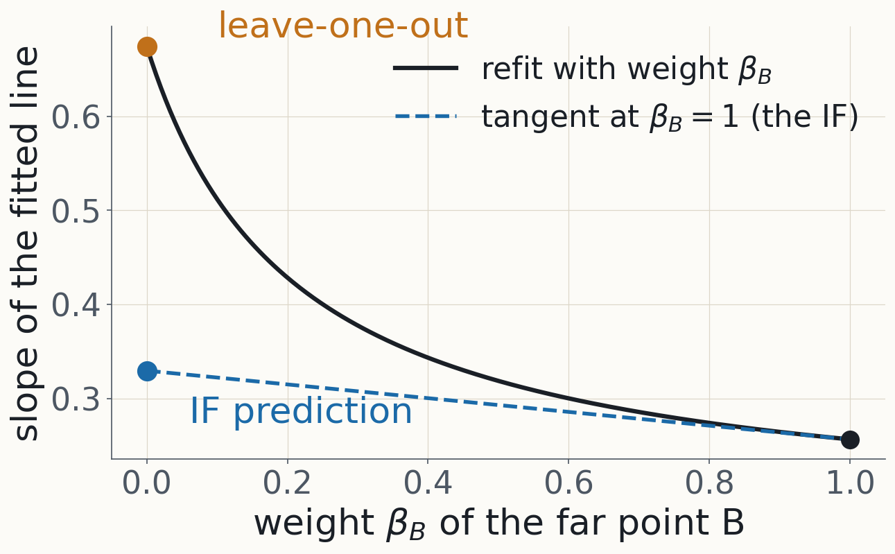
Slope of a regression fit as one point's weight goes from 1 to 0: the exact curve, its tangent at 1, and the two endpoints

One point of a 15-point regression: the tangent predicts a change 5.7× too small.

§2 · Takeaway

Influence is the derivative of a behaviour in one example's weight, through a chosen $\pi$.

§3 · The classical influence function

If training lands at a minimum, where does the minimum go when you reweight one example?

§3 · Warm-up

The influence of a point on a mean

$$\begin{aligned} L(\mu;\beta)&=\tfrac12\textstyle\sum_j\beta_j(z_j-\mu)^2\\[4pt] \htmlClass{fragment}{\mu(\beta)}&\htmlClass{fragment}{=\frac{\sum_j\beta_jz_j}{\sum_j\beta_j}}\\[4pt] \htmlClass{fragment}{\frac{\partial\mu}{\partial\beta_i}\Big|_{\mathbf 1}}&\htmlClass{fragment}{=\frac{z_i-\bar z}{n}} \end{aligned}$$

A point's pull on the mean is its distance from the mean, over $n$.

§3 · The general case

The trained model is defined by an equation

$$\nabla_wL\big(w^*(\beta);\beta\big)=0\quad\text{for all }\beta\text{ near }\mathbf 1$$

Implicit function theorem: if $H=\nabla^2_wL$ is invertible at $w^*$, this defines a smooth $w^*(\beta)$.

So differentiate the equation, not the training algorithm.

§3 · Differentiate in $\beta_i$

Two places $\beta_i$ enters

$$\nabla_wL(w;\beta)=\textstyle\sum_j\beta_j\nabla L_j(w)$$

$$\underbrace{\nabla^2_wL\;\frac{\partial w^*}{\partial\beta_i}}_{\text{through }w^*}\;+\;\htmlClass{fragment}{\underbrace{\nabla L_i(w^*)}_{\text{explicitly}}}\;=\;0$$

At $\beta=\mathbf 1$: $H=\nabla^2_wL(w^*;\mathbf 1)$ is the Hessian, $g_i=\nabla L_i(w^*)$ is $i$'s gradient.

§3 · Solve

The influence function

$$\frac{\partial w^*}{\partial\beta_i}=-H^{-1}g_i\qquad\htmlClass{fragment}{\boxed{\;\mathcal I_i=-\,g_\phi^\top H^{-1}g_i\;}}$$

$g_\phi=\nabla\phi(w^*)$; the chain rule through $\phi$. Needs $H$ invertible.

§3 · Check

It recovers the warm-up

$$H=n,\quad g_i=-(z_i-\bar z)\quad\Longrightarrow\quad -H^{-1}g_i=\frac{z_i-\bar z}{n}$$

For the mean, $L_i=\tfrac12(z_i-\mu)^2$.

§3 · Read it right to left

$H^{-1}$ turns a pull into a move

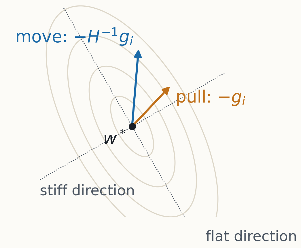
$Contours of an elongated quadratic bowl; the pull -g_i points mostly along the stiff direction, the move -H^{-1} g_i is rotated toward the flat direction$

Flat directions move most. Then $g_\phi$ reads off what $\phi$ cares about.

§3 · What the theorem gives

A local branch, not "the retrained model"

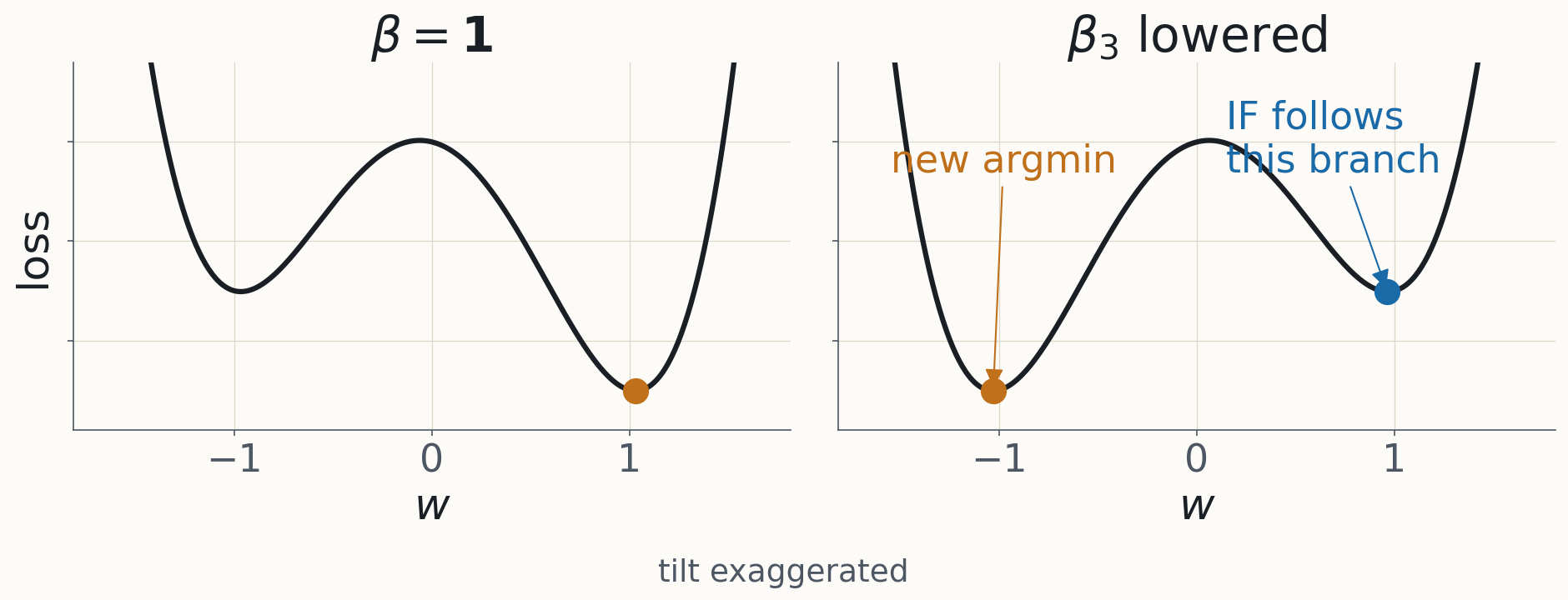
A double well; lowering one example's weight tilts it so the global minimum jumps to the other well while the influence function follows the local branch

The IF follows the nearby minimum; retraining from scratch may land in another basin.

§3 · Takeaway

One linear solve per query: $\mathcal I_i=-g_\phi^\top H^{-1}g_i$.

§3 · How good is it?

How well does a derivative predict deleting a whole example?

§3 · Least squares

Everything is explicit

$$L_j=\tfrac12(y_j-w^\top x_j)^2,\qquad A=\sum_jx_jx_j^\top$$ $$\htmlClass{fragment}{H=A,\qquad g_j=-x_j\,r_j,\qquad r_j=y_j-x_j^\top w^*}$$

The IF says deleting $j$ moves the fit by $-A^{-1}x_j\,r_j$.

§3 · Exact deletion, step 1

Subtract the two sets of normal equations

$$\begin{aligned} \text{all data:}&\quad A\,w^*=\textstyle\sum_ix_iy_i\\[4pt] \htmlClass{fragment}{\text{without }j\text{:}}&\quad\htmlClass{fragment}{(A-x_jx_j^\top)(w^*+\delta)=\textstyle\sum_ix_iy_i-x_jy_j}\\[4pt] \htmlClass{fragment}{\text{subtract:}}&\quad\htmlClass{fragment}{A\,\delta=x_j\,\big(\underbrace{x_j^\top\delta-r_j}_{=:\,c}\big)} \end{aligned}$$

$\delta=w^*_{(-j)}-w^*$ is the exact change. So $\delta=c\,A^{-1}x_j$: only the size $c$ is unknown.

§3 · Exact deletion, step 2

Find the size from its own definition

$$\begin{aligned} x_j^\top\delta&=c\;\underbrace{x_j^\top A^{-1}x_j}_{h_j}\\[4pt] \htmlClass{fragment}{c}&\htmlClass{fragment}{=h_j\,c-r_j\quad\Longrightarrow\quad c=-\frac{r_j}{1-h_j}} \end{aligned}$$

$h_j$ is the leverage of example $j$.

§3 · The result

Exact deletion is the IF, magnified

$$w^*_{(-j)}-w^*=-\frac{A^{-1}x_j\,r_j}{1-h_j}$$

$$\frac1{1-h_j}=\underbrace{1}_{\text{IF}}+\,h_j+h_j^2+\cdots$$

§3 · Leverage

How far a point sticks out, in the data's own metric

$$h_j=x_j^\top A^{-1}x_j\in[0,1],\qquad\sum_jh_j=p$$

$p$: the number of parameters. At $h_j=1$ the point alone pins down a direction.

§3 · The puzzle, solved

Low leverage: close. High leverage: far too small.

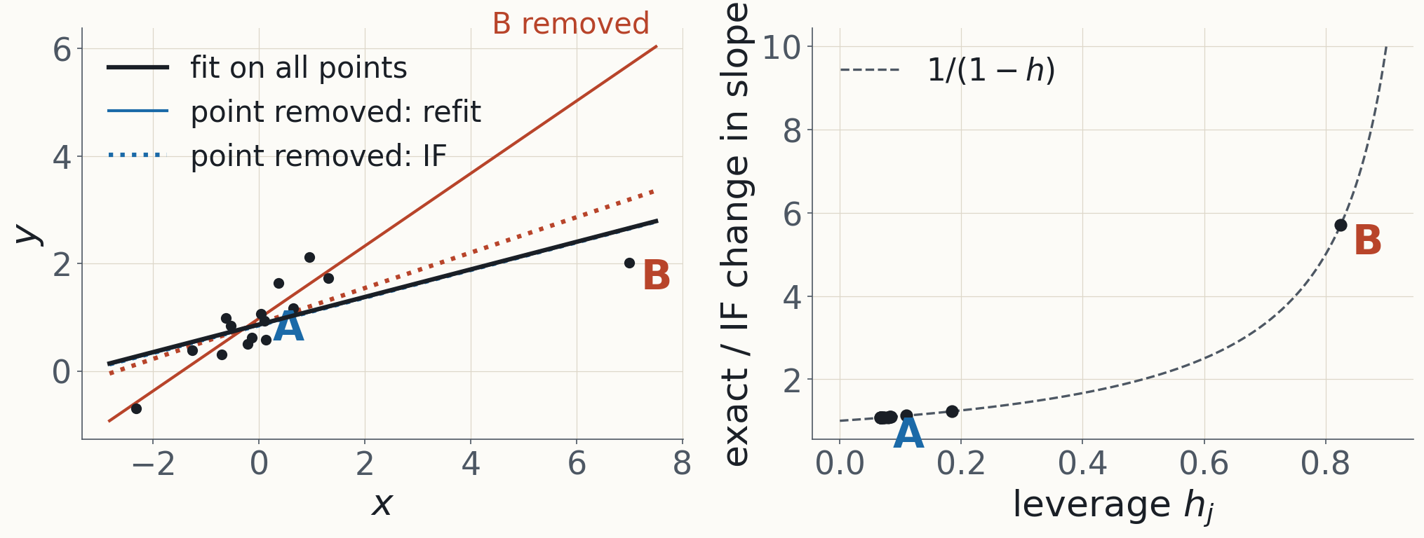
Left: a regression with points A (in the bulk) and B (far out); removing A, refit and IF prediction coincide; removing B, the IF line moves much less than the refit. Right: exact over predicted change against leverage, on the curve 1/(1-h)

Point B has leverage $h=0.825$, so $1/(1-h)=5.7$: the puzzle from slide 15.

§3 · Takeaway

The IF is least reliable for exactly the points you most want to ask about. And this model is convex and converged.

§4 · Neural networks

At a network checkpoint, which assumptions survive?

$H$ invertible? No: flat directions.
$H$ positive? No: negative curvature.
$\nabla L=0$? No: training stopped early.

§4 · Fix 1 · Flat directions

Symmetries make valleys of minimizers

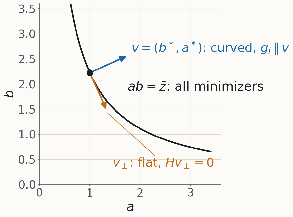
The hyperbola ab = mean of z in the (a,b) plane; at a minimizer, v points across the valley and v-perp along it

A toy: predict $ab$, losses $L_i=\tfrac12(z_i-ab)^2$. Along the valley, $H$ has a zero eigenvalue.

§4 · Fix 1 · Damping

Damping is exact for a proximal question

$$L(w;\beta)+\frac\lambda2\|w-w^*\|^2\quad\htmlClass{fragment}{\xrightarrow{\ \text{Hessian at }w^*\ }\quad H+\lambda I}$$

$$\mathcal I_i^{\lambda}=-\,g_\phi^\top(H+\lambda I)^{-1}g_i$$

Not a numerical patch: reweight $i$, while paying to move away from $w^*$.

§4 · Fix 1 · The toy, by hand

The gradient points across the valley

$$H=n\,vv^\top,\quad g_i=-(z_i-\bar z)\,v\quad\htmlClass{fragment}{\Longrightarrow\quad\mathcal I^\lambda_i=\frac{(z_i-\bar z)\;g_\phi^\top v}{n\|v\|^2+\lambda}}$$

$g_i$ has no flat component, so $\lambda\to0$ is finite. For $\phi=ab$ the limit is $(z_i-\bar z)/n$: the mean again.

In general, in $H$'s eigenbasis $(s_k,u_k)$, $(H+\lambda I)^{-1}g_i=\sum_kc_ku_k/(s_k+\lambda)$ with $g_i=\sum_kc_ku_k$. On a flat direction ($s_k=0$) the factor is $1/\lambda$, which matters only if $c_k\neq0$; then the response grows like $1/\lambda$. If $g_i$ has no flat component, the $\lambda\to0$ limit is the pseudoinverse answer $-H^+g_i$.

$v=(b^*,a^*)$ is an eigenvector of $H$ with eigenvalue $n\|v\|^2$, so $(H+\lambda I)^{-1}v=v/(n\|v\|^2+\lambda)$. $g_i$ is parallel to $v$: no flat component, so nothing diverges.

For $\phi=ab$ (what the model computes, constant along the valley), $g_\phi^\top v=\|v\|^2$ and the limit $(z_i-\bar z)/n$ is the same at every minimizer. For $\phi=a^2$, $g_\phi=(2a^*,0)$, $g_\phi^\top v=2a^*b^*$, and the limit $2\bar z(z_i-\bar z)/(n\|v\|^2)$ depends on the minimizer.

Picked up in: DA1 Exercise 4.1.

§4 · Fix 1 · Where you stand matters

Finite limits, but which one?

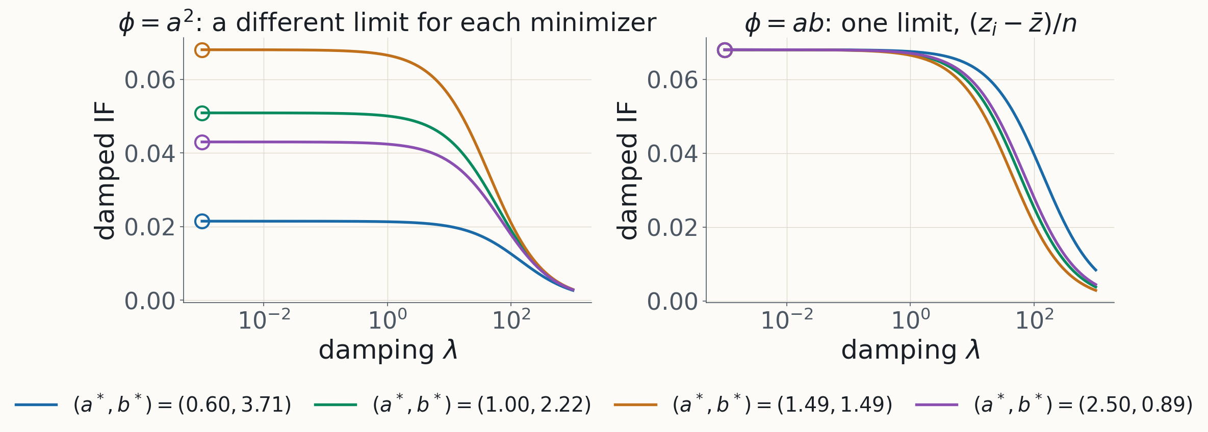
Damped IF against lambda for four minimizers: for phi = a squared the plateaus differ by minimizer; for phi = ab they coincide

$\phi=a^2$ changes along the valley: its answer depends on the minimizer.

§4 · Fix 2 · Negative curvature

Split the Hessian through the outputs

$$L=\sum_i\ell_i\big(f_i(w)\big),\qquad\nabla L=\sum_iJ_i^\top\,\nabla_f\ell_i$$

$$H=\htmlClass{fragment}{\underbrace{\sum_iJ_i^\top H_{y,i}\,J_i}_{G\text{, Gauss–Newton}}}\;\htmlClass{fragment}{+\;\underbrace{\sum_{i,c}\frac{\partial\ell_i}{\partial f_{ic}}\,\nabla^2_wf_{ic}}_{\text{residual term}}}$$

$f_{ic}$: output $c$ on example $i$. $J_i=\partial f_i/\partial w$. $H_{y,i}=\nabla^2_f\ell_i$. Product rule: two terms.

§4 · Fix 2 · Why $G$

$G$ can't have negative eigenvalues

$$\ell_i\text{ convex in }f\ \Longrightarrow\ G\succeq0\ \Longrightarrow\ G+\lambda I\succ0\ \text{ for every }\lambda>0$$

With $H$, an eigenvalue $s<0$ makes $1/(s+\lambda)$ blow up at $\lambda=-s$.

§4 · Fix 3 · Non-convergence

The checkpoint need not minimize the training loss.

So what is $-g_\phi^\top(G+\lambda I)^{-1}g_i$ the derivative of?

§4 · Fix 3 · A tool

The Bregman divergence: the gap above the tangent

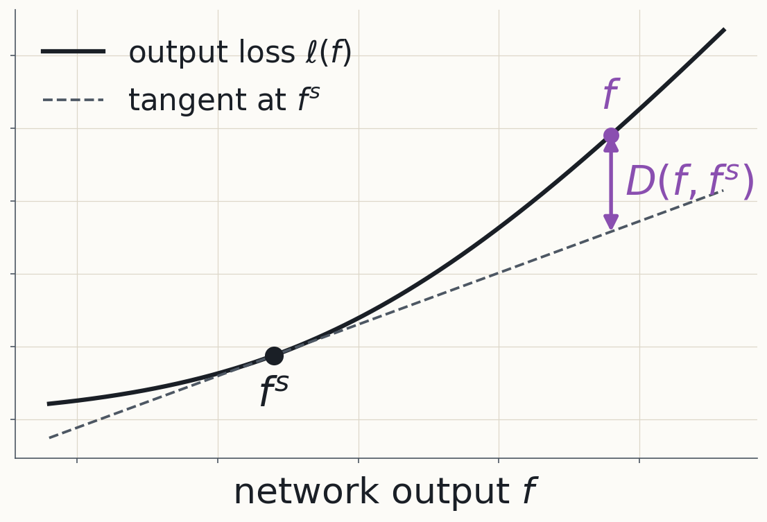
A convex loss curve with its tangent at f^s; the vertical gap between curve and tangent at f is D(f, f^s)

$f^s$: the checkpoint's outputs. $D(f,f^s)=\ell(f)-\ell(f^s)-\nabla\ell(f^s)^\top(f-f^s)$: zero gradient at $f^s$, Hessian $H_y$.

§4 · Fix 3 · The PBRF

Reweight, paying for every move

$$Q(w;\beta)=\underbrace{\sum_j(\beta_j-1)\,L_j(w)}_{\text{the reweighting}}\htmlClass{fragment}{+\underbrace{\sum_jD_j\big(f_j(w),f_j(w^s)\big)}_{\text{output cost}}}\htmlClass{fragment}{+\underbrace{\tfrac\lambda2\|w-w^s\|^2}_{\text{weight cost}}}$$

$w^s$: the saved checkpoint. The minimizer of $Q$ is the proximal Bregman response function, PBRF$(\beta)$.

§4 · Fix 3 · Apply §3 to $Q$

The checkpoint is optimal by construction

$$\begin{aligned} Q(w;\mathbf 1)&=\textstyle\sum_jD_j+\frac\lambda2\|w-w^s\|^2\ \ge0,\ \text{ with equality at }w^s\\[4pt] \htmlClass{fragment}{\nabla^2_wQ(w^s)}&\htmlClass{fragment}{=\textstyle\sum_jJ_j^\top H_{y,j}J_j+\lambda I=G+\lambda I}\\[4pt] \htmlClass{fragment}{\partial_{\beta_i}\nabla_wQ}&\htmlClass{fragment}{=\nabla L_i(w^s)=g_i} \end{aligned}$$

No residual term: $D_j$ has zero gradient in $f$ at $f^s$.

§4 · Fix 3 · The result

The practical formula, and its question

$$\frac{\partial\,\phi\big(\mathrm{PBRF}(\beta)\big)}{\partial\beta_i}\bigg|_{\beta=\mathbf 1}=-\,g_\phi^\top(G+\lambda I)^{-1}g_i$$

Exact, for a question that isn't retraining. Slide 3's LLM results used an approximation of it.

§4 · The proximity gap, measured

The damped IF answers its own question

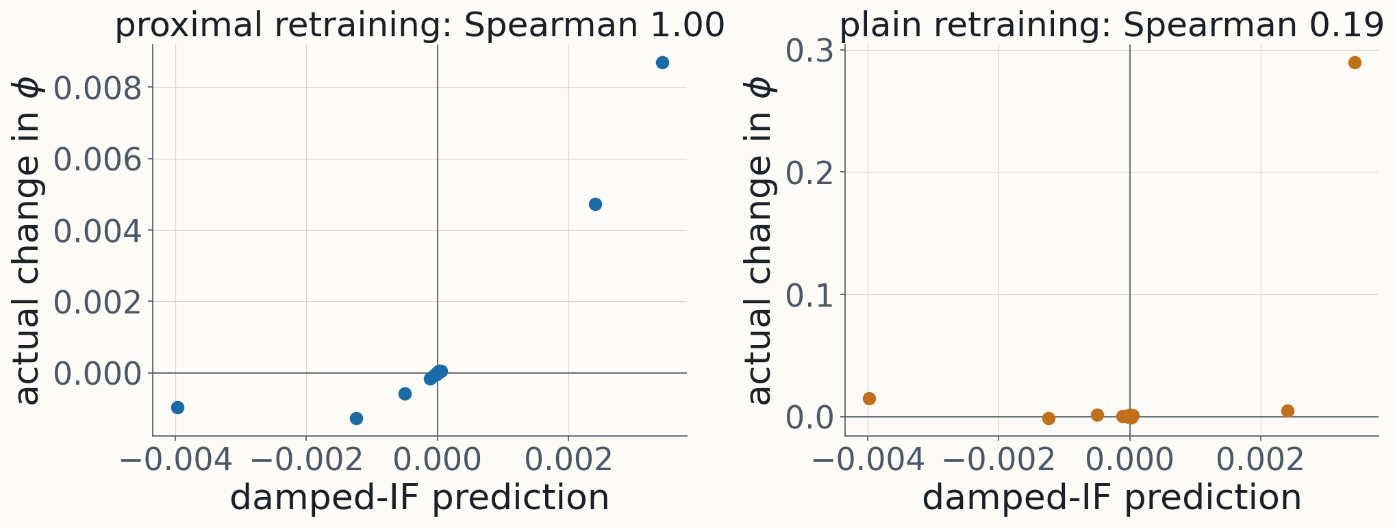
Two scatter plots for a 25-parameter MLP: damped-IF predictions against proximal retraining (Spearman 1.00) and against plain retraining (Spearman 0.19)

A 25-parameter MLP: it ranks proximal retraining almost perfectly, plain retraining hardly at all.

Note: this experiment uses the damped Hessian IF of slide 36, $-g_\phi^\top(H+\lambda I)^{-1}g_i$, not Gauss–Newton. The training objective includes a fixed ridge $\frac{10^{-3}}2\|w\|^2$ in every refit, and $H$ includes it. Spearman for proximal retraining is 0.995.

This is one of five gaps Bae et al. identify between the IF and leave-one-out retraining. Changes of question: warm start (retraining starts from $w^s$, not a fresh init), proximity (moving the parameters is penalized), non-convergence (the Bregman term stands in for the loss). Errors: linearization, the approximate solve. For networks the changes of question dominate (their Fig. 4).

One hidden layer of 8 tanh units, 20 noisy points of $\sin2x$, trained to a minimum by Newton's method; $\phi$ is the squared error at one test input; $\lambda$ is 1% of the top Hessian eigenvalue. Deleting each point: damped-IF prediction vs proximal retraining (the IF's own target, made finite) vs plain retraining from $w^*$.

The Hessian's eigenvalues run from $5\times10^{-4}$ to 106: without the proximal term, a deletion moves the parameters far along nearly flat directions (across deletions, the vector of plain-retraining changes has 49 times the norm of the IF predictions). Which one you want is a choice of question, not a matter of accuracy.

Picked up in: DA1 §4 extension.

§4 · Takeaway

Each fix changes the question. The damped Gauss–Newton IF answers the PBRF question exactly.

§5 · Checking

How would you know an attribution is right?

§5 · Two separate things

Target and estimator

Target: the question. A choice of $\pi$, and of one of the three targets.
Estimator: how you compute the answer.
They fail separately, so they need separate checks.

§5 · Three checks

From least to most demanding

Finite differences of the method's own target.
Leave-one-out retraining.
Retraining on random half-subsets.

§5 · The linear datamodeling score

Do summed scores order the subsets?

$$\mathrm{LDS}=\mathrm{Spearman}\Big(\big\{\phi(S_k)\big\},\ \Big\{\textstyle\sum_{i\in S_k}\mathcal I_i\Big\}\Big)$$

$S_k$: a random half of the data; retrain on it and measure $\phi(S_k)$. It checks the ranking, not the size.

§5 · One example

Different checks rank methods differently

	1: own target, rel. error	2: LOO, Spearman	3: LDS
exact IF	$3\times10^{-7}$	0.96	0.83
damped IF	$3\times10^{-7}$ (proximal)	0.82	0.83
gradient dot product	—	0.36	0.56

Both IFs nail their own target; LOO prefers the exact IF; LDS can't tell them apart.

Logistic regression, $n=80$: pick the check that matches your question. DA1 §5's setup: $\ell_2$-regularized logistic regression, 80 examples in 10 dimensions with feature scales spanning 1.5 decades, 10 test losses as observables; Newton solver, so every check is deterministic. Damping $\lambda$ = median Hessian eigenvalue.

The damped IF is off by 48% against the plain local derivative, but matches its own proximal target to $3\times10^{-7}$: a different target, not a defect. It is worse on LOO and ties on LDS. Calibration slopes on the half-subsets are 12 to 35, far from 1: a high LDS doesn't license "deleting these changes the loss by this much".

The gradient dot product ignores the $H^{-1}$ rotation of slide 23; the Hessian's eigenvalues here span a factor of about 360.

Picked up in: DA1 Exercises 5.1–5.2, where you compute this table.

§6 · Another $\pi$

What if $\pi$ is this training run, not an argmin?

§6 · A lens

Many estimators filter the curvature spectrum

$$\frac{\partial w}{\partial\beta_i}=-F(M)\,g_i=-\sum_kF(s_k)\,c_k\,u_k$$

Classical IF: $F(s)=1/s$. Damped: $1/(s+\lambda)$. Now one more.

§6 · Unroll gradient descent

Differentiate $K$ steps instead of an argmin

$$\begin{aligned} r_t&=\partial w_t/\partial\beta_i,\qquad w_{t+1}=w_t-\eta\nabla_wL(w_t;\beta)\\[4pt] \htmlClass{fragment}{r_{t+1}}&\htmlClass{fragment}{=(I-\eta H)\,r_t-\eta\,g_i,\qquad r_0=0}\\[4pt] \htmlClass{fragment}{r_K}&\htmlClass{fragment}{=-\eta\textstyle\sum_{k<K}(I-\eta H)^k\,g_i}\\[4pt] \htmlClass{fragment}{F(s)}&\htmlClass{fragment}{=\eta\textstyle\sum_{k<K}(1-\eta s)^k=\dfrac{1-(1-\eta s)^K}{s},\qquad F(0)=\eta K} \end{aligned}$$

Constant curvature and gradient give a geometric series; per eigenvalue, a filter.

§6 · The filters

Same shape, different meanings

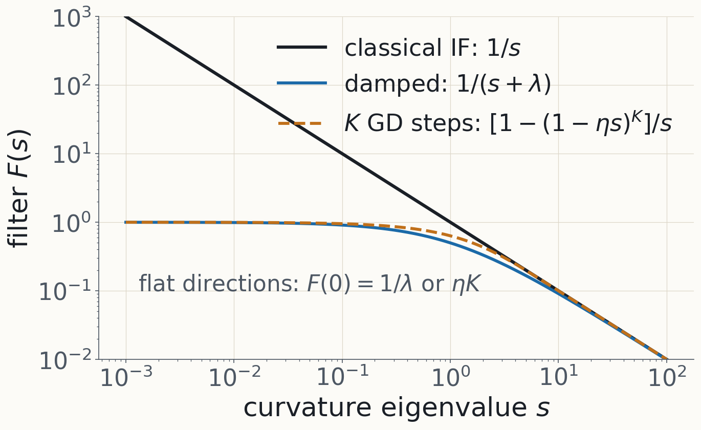
Log-log plot of filters: 1/s diverges at small s; the damped filter and the K-step GD filter flatten to a finite value

$\lambda$ is a proximal penalty; $\eta K$ is training time. Both tame the flat directions.

§6 · The afternoon's map

DA2's methods differ mainly in what $\pi$ is

method	$\pi(\beta)$ is
classical IF	the stationary point near the trained $w^*$
PBRF	a proximal optimum around the checkpoint
unrolling	this run's last iterate, same seed and order
Bayesian IF	a local posterior
datamodels	a fitted predictor of retraining

§6 · Takeaway

Training time can play the role of damping. Same shape, different question.

Takeaway

Before trusting an attribution, ask which $\pi$, which target, and which check.

The day

How to use the day

Morning: DA1, §1–§6. Do Exercises 3.1, 5.1 and 5.2.
After lunch: L2, curvature at scale.
Then: the DA2 tour. Read each capsule; go deep anywhere.

Readings · Importance / Length

Koh & Liang 2017, Understanding Black-box Predictions via Influence Functions ●●●●● / ●●○○○
Bae et al. 2022, If Influence Functions are the Answer, Then What is the Question? ●●●●● / ●●●○○
Grosse et al. 2023, Studying LLM Generalization with Influence Functions ●●●●● / ●●●●○
Park et al. 2023, TRAK: Attributing Model Behavior at Scale ●●●●○ / ●●●○○
Mueller 2024, Missed Causes and Ambiguous Effects ●●●○○ / ●●○○○